Field Notes

JUBAP.NET Field Notes · Case Study · Distributed American Innovation

The Tuxpan Urban Mobility Case: Operational Intelligence Before the Platform Era

A case study in constraint-driven architecture, hybrid formal–informal mobility ecosystems, and pan-American operational intelligence — fifteen years before agentic orchestration became a category.

NodeJUBAP.US · Americas Integration Unit
Field Period2010–2011
LocationTuxpan, Veracruz, MX
Fleet Scope≈60 units · ≈70% urban coverage
SystemsGPS · GPRS · CV counting · Control Center
SeriesFrontier Engineering Cases
SUT urban transport fleet, Tuxpan, Veracruz
Field record. Servicio Urbano de Tuxpan (SUT): a concession-based bus network operating in permanent competition with an informal collective-taxi ecosystem, Gulf of Mexico corridor, 2010.
Thesis Some of the most valuable operational intelligence architectures did not emerge from idealized smart-city environments. They emerged from constrained hybrid ecosystems where formal and informal systems had to coexist under real economic pressure — and where technology’s job was not to replace distributed human intelligence, but to stabilize it.

This case study is not only about a transportation system. It is about how innovation emerges when formal infrastructure, informal intelligence, human incentives, and hard technological constraints collide in the real world.

The JUBAP.US node was built around a simple but demanding idea: American innovation is distributed. Not all of it emerges from corporate laboratories, universities, or well-funded technology ecosystems. Across the Americas, operational innovation has repeatedly emerged from cities, borders, ports, transport corridors, industrial sites, and informal economies — environments where people must solve real problems continuously, with whatever is at hand. In that sense, Latin America is not merely a market for imported innovation. It is a living laboratory of adaptive systems.

The case below focuses on one concrete example: urban transport intelligence in Tuxpan, Veracruz, developed after earlier field learning in Cuba and before large-scale mobility platforms became mainstream. The claim is precise: many patterns later formalized by digital platforms already existed as human, operational, and informal coordination mechanisms in Latin American environments. The work documented here consisted of understanding those patterns, extracting their operational intelligence, and translating them into usable architecture.

Section 01From Barcelona to Cuba: The First Operational Shock

Before the Mexican field work, a formative experience took place in Cuba, at the University of Las Tunas. It was framed as a teaching mission; in practice it was a learning experience.

The mental model arriving from Barcelona was European transport planning: structured public transport, frequency control, multimodal ticketing, planned routes, centralized coordination. Barcelona had demonstrated that a city could solve much of its mobility problem through architecture — integrated routes, shared tickets, intermodal connections.

Cuba revealed something different. Transport operated through an extraordinary mix of modes: buses, trucks adapted for passengers, collective taxis, motorcycles, bicycles, horse carts, informal shared rides. At first sight, disorder. Operationally, something deeper: a highly adaptive mobility ecosystem that ran not on formal infrastructure but on human coordination, negotiation, local knowledge, and continuous adaptation.

One concrete pattern stood out: the collective taxi model. A passenger could sponsor a trip by agreeing to pay the full ride. Along the way, the driver picked up additional passengers heading in the same direction, each paying a smaller amount. If enough passengers joined, the original sponsor paid only for their own seat. No app, no algorithm — yet conceptually the pattern already contained dynamic demand aggregation, shared-ride economics, on-demand routing, and flexible cost distribution. Modern platforms later formalized these ideas through GPS and payment systems. The operational pattern preceded them.

Field Lesson Innovation does not always start as software. Sometimes it starts as a social protocol.

Section 02Tuxpan: A Hybrid Mobility Ecosystem

Tuxpan, a mid-sized port city on the Veracruz coast, became the environment where these lessons were tested. The city had a formal bus system — Servicio Urbano de Tuxpan — operating roughly sixty units under a concession structure and covering around seventy percent of the city’s neighborhoods. In parallel, a strong informal collective-taxi ecosystem operated on the same demand.

The formal system had established routes, expected frequencies, and public service responsibilities. But actual behavior was more complex. Most drivers did not operate under a simple salaried logic; income depended on passengers collected and route economics. In practice, each driver behaved as a semi-autonomous operator inside a formal network — and that created a structural incentive problem.

If buses were supposed to pass every five minutes, a stable system would maintain even spacing. But a bus arriving right behind another found fewer passengers; a bus delaying slightly captured more demand near schools, markets, and the city center. Drivers therefore had rational incentives to distort spacing. And when delays grew too large, a second system reacted.

Section 03The Taxi Swarm as an Informal Intelligence Layer

The informal taxi ecosystem did not compete as a fixed-route network. It behaved like a swarm. It detected gaps: when buses delayed, passengers accumulated at stops; once waiting became uncomfortable, taxis entered the gap, collected the most urgent passengers into informal collective rides, and left.

In architectural terms, the swarm acted as an elasticity layer, a demand-overflow mechanism, a real-time gap filler. It was reading the system continuously — where passengers were waiting, where buses were late, where frustration was rising, where collective rides became profitable. The system was informal, but it was intelligent.

The problem was that this intelligence also destabilized the formal network. Buses that delayed to capture demand lost it to taxis if they delayed too much. Buses competing with each other broke frequency; broken frequency eroded passenger confidence; eroded confidence made taxis more attractive. The result was not «formal versus informal.» It was a multi-agent mobility ecosystem with competing incentives — swarm instability in the literal sense.

Section 04The Real Architectural Problem: Incentives, Not Routes

Most transport projects treat routes as the main problem. In Tuxpan, routes mattered, but the deeper problem was incentive architecture. Why would a driver respect frequency if breaking it increased income? Why would a driver report overcrowding accurately if standing passengers meant revenue? Why would informal taxis disappear while they were filling real service gaps? Why would a rigid European-style system work without adapting to local behavior?

The transport system was not only infrastructure. It was a living economic system. The solution therefore could not be purely administrative, and it could not be purely technological. The challenge was to introduce enough intelligence and governance to stabilize the system without destroying the adaptive flexibility that already existed.

Section 05The Architectural Synthesis: Four Operational Cultures

The solution did not copy one model. It combined elements from four operational worlds into a single practical architecture:

Barcelona

  • Multimodal integration
  • Ticket-based transfer logic
  • Frequency control
  • Formal route architecture

Cuba

  • Adaptive intermodality
  • Demand aggregation
  • Shared-ride logic
  • Respect for informal coordination

Mexico

  • Formal–informal coexistence
  • Route competition dynamics
  • Low-cost implementation
  • Field-based adaptation

Early Platform Thinking (US)

  • GPS-based control
  • Telemetry and distributed devices
  • Extensible onboard platforms
  • Control-center coordination

The goal was never to impose a foreign model. It was to build an architecture that could operate in the real city.

Section 06Implementation I — A Low-Tech Multimodal Ticket

The first implementation addressed network expansion. A new feeder line was needed to serve a poorly connected neighborhood, but demand was insufficient for a direct route. The real friction was not the route itself: passengers wanted to reach the city center, and transferring between lines meant paying twice. Double payment made the new line unattractive; low attractiveness kept frequency low; low frequency kept the neighborhood disconnected.

The classic European answer — electronic validation, smart cards, integrated ticketing infrastructure — was impossible. The buses had no such technology and the budget did not allow it. So the question was reframed:

Reframing Not «how do we install a modern ticketing system?» but «how do we create transfer rights without digital infrastructure?»

The answer was a ticket designed to be cut or manually marked, representing a valid same-day transfer, with day-coded colors making it visually verifiable. Drivers validated transfers without any electronic system. In the final implementation, a simple manual cut on the ticket. It worked, and the feeder line connected the neighborhood to the broader network.

The innovation was not the paper ticket. It was architectural: interoperability without digital infrastructure; transfer rights without electronic validation; network expansion without CAPEX; human-readable distributed state management. The ticket carried valid state — authorization, temporality, transfer rights — in a form that was cheap, robust, trainable, and failure-resistant. Constraint-driven architecture in its purest form.

Section 07Implementation II — Passenger Counting by Computer Vision

The second implementation addressed observability. Frequency decisions required knowing how full buses actually were — but asking drivers was unreliable, because drivers had limited incentive to report overcrowding when additional passengers meant additional income. A governance problem, stated plainly: the system needed observability independent of the operator’s incentives.

Physical turnstiles were tested conceptually and rejected: in a fast, agile Mexican boarding environment, turnstiles destroyed throughput. The control mechanism damaged the very flow it was supposed to govern — a failure mode common to formalist systems that optimize control at the expense of operation.

The path taken instead was camera-based passenger counting. Around 2010, the technology was imperfect and the margin of error significant. But perfect accuracy was never the requirement. The system only needed to distinguish whether a bus was nearly empty, reasonably loaded, overcrowded, or operating outside expected patterns. That was enough to support frequency decisions.

Core Principle Operational intelligence does not require perfect data. It requires sufficient signal quality, actionable visibility, and adaptive decision capability.

In modern language, this was an early observability layer for public transport operations — good-enough telemetry serving as governance infrastructure where previously there was only driver reporting, passenger complaints, and intuition.

Section 08Implementation III — GPS, SIM Connectivity, and Micro-PC Fleet Intelligence

The third implementation was onboard route and frequency control. In 2010, the device decision was not obvious. Smartphones were immature: Android was early, the iPhone expensive, sensors limited, the ecosystem unstable. Integrated boards and Arduino-type approaches were explored, but deployment pressure demanded speed and reliability. The practical answer was low-cost industrial micro-PCs.

Each onboard unit combined a small PC, USB-connected GPS/SIM device, mobile GPRS connectivity, camera integration, and the capacity to transmit position and operational data to a control center — initially on Windows, with Linux alternatives evaluated. Full unit cost, including camera and connectivity: roughly 200–300 euros.

This was not a GPS tracker. It was an extensible onboard computing platform — a base for passenger information, maintenance telemetry, future sensors, local processing, and operational alerts. Platform thinking before platformization became mainstream; edge intelligence before «edge computing» entered the urban transport vocabulary. The bus became a connected operational node.

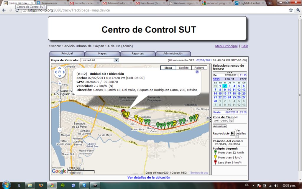
SUT Control Center — unit tracking view with GPS position, speed, and odometer
Fig. 1 — SUT Control Center, unit view (2010–2011). Live GPS position, speed, altitude, odometer, heading, and time-stamped events per identified unit, coordinated from a central operations console.
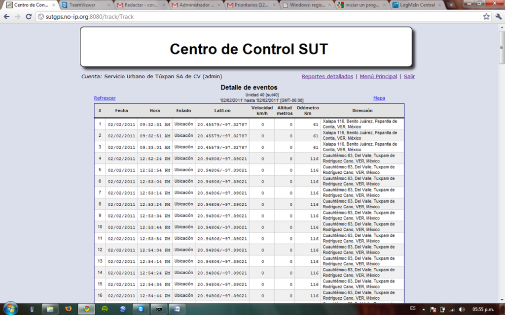
SUT Control Center — operational map and detailed event report
Fig. 2 — SUT Control Center, operational map and event log. Fleet traceability and historical event reporting: an early low-cost mobility intelligence layer for a mid-sized Latin American city — not a concept deck, a running system.

Section 09Competing With the Swarm Through Intelligence

The purpose of the system was not surveillance of buses. It was to let the formal network compete intelligently with the informal swarm. The swarm’s advantage was real-time responsiveness. The bus system’s weakness was poor visibility and distorted incentives. Onboard intelligence changed that balance.

With GPS, passenger counting, and control-center visibility, the operator could see where each bus was, where frequency gaps were emerging, which buses were saturated or underused, where passenger accumulation was likely, whether drivers were distorting spacing, and where a route was vulnerable to taxi capture. The control center could then instruct drivers to slow down, speed up, hold spacing, and protect key demand points.

Design Intent Intelligence was used to reduce destructive competition without destroying adaptive flexibility. Too much freedom produced chaos; too much control produced rigidity. The system’s target was dynamic equilibrium.

The vocabulary is contemporary — adaptive orchestration, real-time telemetry, swarm coordination, distributed optimization — but the deployment was fifteen years earlier, in a constrained Latin American environment, with resources measured in hundreds of euros per node. Alongside the technical layer ran an explicit cultural change programme for operators, launched in September 2010: process, training, and incentive alignment were treated as part of the architecture, not as an afterthought.

Section 10What Was Actually Learned

The most important learning was not technical. It was architectural.

  1. Informal systems often contain real intelligence.

    What looks like disorder may be a highly adaptive pattern that formal systems fail to see. Dismissing it discards operational knowledge.

  2. Technology should stabilize intelligence, not replace it.

    The goal was never to replace drivers, passengers, or local practice — it was to make the system visible, fair, and coordinated.

  3. Good-enough telemetry creates major operational value.

    Perfect data was not needed. Sufficient signal quality for better decisions was.

  4. Low-tech architecture can solve high-impact problems.

    A cut in a paper ticket solved a network-integration problem that would otherwise have required electronic ticketing infrastructure.

  5. Mobility is an incentive system.

    Routes, vehicles, and tickets matter — but incentives explain behavior. Governance is part of the architecture.

  6. Latin America is an adaptive-systems laboratory.

    Constrained environments force innovation that rarely looks like formal R&D, yet often contains deep operational intelligence.

Section 11Why This Matters: Distributed American Innovation

JUBAP.US was never just a technology node. It represented a working philosophy: innovation across the Americas is not centralized in one country, one city, one laboratory, or one type of institution. It emerges from Barcelona-style urban architecture, Cuban adaptive mobility, Mexican field constraints, US platform thinking, and Latin American operational creativity — and its integration happens through people who move between these worlds and translate field intelligence into practical architecture.

The case is relevant today because current discussions around AI, mobility platforms, and agentic systems tend to assume that intelligence must be centralized, digital, and algorithmic. Tuxpan shows something different: before software platforms became dominant, human ecosystems were already performing distributed intelligence — adaptive routing, demand aggregation, swarm response, real-time rebalancing, decentralized decision-making. The architectural challenge is not only to automate these systems. It is first to understand them, and then, where useful, to formalize them carefully.

That discipline — reading real operational behavior before designing the intelligence layer above it — is the same discipline that today underpins JUBAP.Net’s work in Operational AI Integrity and early-warning regime change detection. The Tuxpan case is one of its field origins.

Operational Lineage

Barcelona (multimodal architecture) → Las Tunas, Cuba (adaptive mobility field learning) → Tuxpan, Veracruz (constraint-driven fleet intelligence, 2010–2011) → Gulf Corridor / Pan-American ecosystems (distributed operational integration) → JUBAP.Net (Operational AI Integrity & regime change detection)

Tegrity.AI
Regime-Awareness Programme
Code-grounded research series
Tegrity.AI · Regime-Awareness Programme

Revision-Aware Event Semantics and Relabeling Cascades

A Code-Grounded Reconstruction of Retrospective Labels, Causal Confirmation, Hierarchical Event Levels, and Selective Rebuilding in JUBAP/Phylons
Bounded rematerialization, event-time / knowledge-time separation, dependency-aware lineage, and conditional quantum triage
Architecture overview for Revision-Aware Event Semantics and Relabeling Cascades
Technical working papercode-grounded edition v2.0July 2026Private preprint
Primary sources: supplied xbot and JUBAP-PFS snapshots; Predictive Factors; JUBAP Libro Blanco; PHYLONS 1–7 with LM 4.x; Papers V and VI.
Iván Abril Palma · IMSV.org / tegrity.ai working group
Central thesis. A relabeling cascade is selective downstream invalidation under explicit event and knowledge versions—not an assumed rebuild of the entire system.

Abstract

This paper reconstructs the revision-aware event substrate of JUBAP/Phylons from two supplied source snapshots and the historical design corpus. The xbot snapshot implements a retrospective path: local extrema are filtered through centred windows, hidden extrema can be recovered, waves and targets are deleted and rematerialized over a bounded recent interval, predictive factors are recalculated with history padding, and materialized factor-state arrays are replaced from the last stored timestamp. The later JUBAP-PFS snapshot implements a causal streaming path: candidate extrema are confirmed only after subsequent evidence, the event is stored at its historical position while confirmation is emitted at the current stream position, higher event levels are constructed recursively, and temporary extrema are represented separately from confirmed ones. Together, these artifacts expose a research object more precise than a generic “relabeling cascade”: a new observation can revise an earlier event in event time, and that revision can propagate forward through the subset of derived objects that actually depend on the event branch.

The paper therefore separates three layers. First, it documents the code-grounded historical mechanisms. Second, it introduces an implementation-ready, dependency-aware reconstruction with versioned event records, knowledge-time cutoffs, selective invalidation, topological rebuilding, and a cascade-cost ledger. Third, it treats quantum computation as a conditional research option rather than an established advantage. Amplitude amplification or amplitude estimation becomes relevant only after a fixed candidate universe, a reversible marking or sampling oracle, coherent state preparation, error targets, and total resource costs are specified. Event detection, feature construction, dependency traversal, and rebuilding remain classical. The strongest contribution is thus classical and falsifiable: an evolution from retrospective event reconstruction to causal event semantics, plus a concrete benchmark for measuring when revisions matter, how far they propagate, and whether any quantum triage layer could ever cross the engineering cost frontier.

Keywords: event semantics; relabeling; causal replay; knowledge time; dependency graph; incremental recomputation; regime detection; quantum amplitude amplification; amplitude estimation

Evidence and terminology discipline

Label Meaning
DESIGN-2018 Directly documented in the historical JUBAP/Phylons design corpus.
CODE-XBOT Directly verified in the supplied xbot source snapshot.
CODE-PFS Directly verified in the later supplied JUBAP-PFS source snapshot.
RECON Executable pseudocode or data structures faithful to the documented or coded behavior.
MATH Formal definition or complexity statement introduced in this paper.
QUANTUM-CANDIDATE A quantum formulation whose end-to-end value requires an oracle and resource ledger.
OPEN Property requiring replay, instrumentation, missing lineage data, empirical fitting, or formal proof.

Contents

  • 1. The problem: provisional meaning and historical revision

  • 2. Evidence base and corrected object model

  • 3. Event-sensitive context architecture

  • 4. Retrospective reconstruction and bounded rematerialization in xbot

  • 5. Causal streaming confirmation and event levels in JUBAP-PFS

  • 6. From event revision to selective relabeling

  • 7. Classical-first dependency-aware rebuilding

  • 8. Measuring cascades and near-degeneracy

  • 9. Conditional quantum triage and the crossover frontier

  • 10. Playable implementation and research programme

  • Appendices: code map, event schema, claim/evidence ledger, references

1. The problem: provisional meaning and historical revision

A numerical observation does not carry its final structural meaning at the instant it arrives. A local maximum can be a temporary high, a confirmed event, or a child of a later higher-level event depending on subsequent observations. The architecture therefore faces two clocks: event time, where the candidate extremum occurred, and knowledge time, when enough evidence existed to use that interpretation. Mixing those clocks creates leakage in replay; keeping them separate creates a revision problem that must be governed explicitly.

A new observation can change an earlier label in event time. That revision does not move backward through computation. It moves forward through the derivation graph: event -> wave or support -> event-sensitive factor -> qualitative state -> context -> detector or rule -> decision record. The historical timestamp is earlier, but the computational dependencies are downstream. This distinction is central to a precise relabeling model.

1.1 Research questions

  • How did the xbot snapshot reconstruct extrema and rematerialize affected waves, targets, and factor-state arrays?

  • How does the later PFS snapshot distinguish historical event position from current confirmation time?

  • Which context branches are event-sensitive, and which can remain valid after an event revision?

  • How should a lineage graph, revision ledger, and replay cutoff be represented so that rebuilding is deterministic and testable?

  • What empirical distribution do cascade size, depth, wall-clock cost, and affected decisions follow?

  • Under which oracle and resource assumptions could a quantum triage layer outperform the best classical scheduler?

1.2 Contribution

  • A code-grounded genealogy from retrospective centred-window labels to causal streaming confirmation and hierarchical event levels.

  • A precise separation between event time, confirmation time, materialization time, and decision cutoff.

  • A branch-selective dependency model that preserves fixed-window, microstructure, and external context when an event-only branch changes.

  • Implementation-ready pseudocode for versioned events, descendant invalidation, topological rebuild, idempotent replay, and cascade accounting.

  • A classical benchmark ladder: full rebuild, bounded time-window rebuild, dependency-aware rebuild, and causal append-plus-revision processing.

  • A conditional quantum formulation with explicit oracle, state-preparation, precision, confidence, and total-cost gates.

2. Evidence base and corrected object model

The earlier draft usefully identified revision as a computational problem, but Papers V and VI now provide a more precise ontology. A predictive factor is not a Phylon. A subpf is a qualitative predicate generated from a factor. A combination is a conjunction of subpf states. A strategy adds explicit negative combination exceptions. A Phylon is a specialized detector that consumes this context substrate for a declared prediction problem and timeframe. The revision paper uses that typed chain throughout.

Source Verified contribution Status
xbot: bot/models/waves.py Centred local/true extrema, bounded recent rematerialization, target persistence, incremental factor recomputation and WavesPF replacement. CODE-XBOT
xbot: performance_c/predictives_factors/truepeak.pyx Hidden-extremum recovery and event-conditioned statistics over truepeak arrays. CODE-XBOT
JUBAP-PFS: app/peaks/peaks_relevant.pyx Streaming relevant extrema, area relevance, confirmation lag, recursive levels, temporary extrema and correspondence helpers. CODE-PFS
JUBAP-PFS: app/peaks/view.py Separate emission of peak_conf at current time and peak/peak_area at historical event time. CODE-PFS
Paper V Typed context objects, 54 factor-family dispatcher, event-sensitive and non-event-sensitive factor families, materialized state. CODE-XBOT / DESIGN-2018
Paper VI Materialized rule search, multi-horizon support, interaction-constrained growth, negative exceptions and incremental maintenance. CODE-XBOT / DESIGN-2018
Historical design corpus Presumed/confirmed events, waves, multiresolution factors, Phylon reversal/recharge distinctions and labeling/relabeling intent. DESIGN-2018

2.1 Four timestamps, not one

Time coordinate Meaning Replay rule
event_time Historical position at which the extremum or event is attached. May be earlier than the time at which the label becomes usable.
confirmation_time Observation time at which the event meets the confirmation rule. The event is unavailable before this cutoff in causal replay.
materialized_at Time at which a derived wave, factor state, or context version is persisted. Used for audit and rebuild ordering.
decision_time Time at which a detector, rule, or operation consumes context. May consume only versions known by this time.

3. Event-sensitive context architecture

Figure 1. The event branch is one source of context, not the
universal origin of every factor. Selective rebuilding can preserve
unaffected branches.
Figure 1. The event branch is one source of context, not the universal origin of every factor. Selective rebuilding can preserve unaffected branches.

Paper V verifies that the context vocabulary is heterogeneous. Morphology, maturity, event regularity, and some range descriptors depend directly on peak/wave structure. Conventional fixed-window indicators can be recomputed from raw bars without a truepeak hierarchy. Order-flow and liquidity geometry originate in order-book and trade data. Calendar, social, market-cap, and Bitcoin-role context have distinct relational sources. All branches are materialized into a common state space, but they do not share the same revision dependency.

Branch Representative objects Revision behavior
Event-sensitive truepeak, wave shape, maturity, event regularity, event-defined range. A revised event can change support, value, state and downstream detector matches.
Fixed-window ROC, RSI, ATR, MACD, Bollinger and similar bar-window transforms. Normally unaffected by an event relabel; may still change when raw data changes.
Microstructure Ask/bid distance, dispersion, active volume, emergent order flow. Depends on order-book/trade corrections, not necessarily on event anchors.
External/relational Hour, weekday, social mentions, market-cap and Bitcoin-state enrichment. Depends on its own source and alignment/version rules.
Materialized context WavesPF active state identifiers, asset role, target outcomes. Must be reassembled under a consistent set of source versions and knowledge cutoff.

3.1 Formal context dependency

Let a materialized context at decision time t be a set of active predicates assembled from several source branches:

C_t^(v) = C_event,t^(v_e) union C_fixed,t^(v_f) union C_micro,t^(v_m) union C_external,t^(v_x)

A revision to event version v_e does not imply that v_f, v_m, or v_x changed. The rebuilt context receives a new aggregate version v, but unaffected branch states can be reused if their source versions and timestamps remain valid. This is the key computational potential of explicit lineage: explainability can reduce work when dependencies are precise.

4. Retrospective reconstruction and bounded rematerialization in xbot

The xbot snapshot contains two related reconstruction paths. WavesQuerySet.frames builds a recent market frame, calculates local extrema, filters them through centred rolling maxima/minima, computes wave fields and configured target outcomes, and replaces Waves and WavesTargets from a bounded apply_change_from_date. For minute periods the window begins five hours before the last persisted wave; for longer periods it begins twenty-four hours before. This is a coarse but operational invalidation boundary.

Artefact 1 — bounded retrospective wave and target replacement

last = Waves(...).order_by('-dt').first() lookback = 5 hours if period is minute-based else 24 hours apply_change_from_date = last.dt - lookback peak = local_extrema(high, low) truepeak = centred_extrema(peak, window=2 * period_truepeak) wave_fields = calculate_wave_state(truepeak, market, order_book) targets = evaluate_all_configured_targets(open, high, low, close) transactionally: delete Waves and WavesTargets from apply_change_from_date bulk_create reconstructed waves and targets
Status: CODE-XBOT / RECON from
bot/models/waves.py: frames. The source uses a concrete recent-time
boundary and transactional delete/bulk-create persistence.

This design has practical value. It avoids relying on a permanently frozen interpretation of the recent boundary, keeps the stored wave table internally coherent, and supplies a deterministic historical reconstruction baseline. It does not preserve decision-time causality because centred extrema use observations to the right of the historical event. That is acceptable for final-label construction provided replay does not expose the final label before it was knowable.

4.1 Hidden-extremum recovery and alternating event structure

The factor-materialization path recalculates truepeak and invokes search_truepeak_hidden. The Cython routine scans the provisional labels, tracks the lowest point after a peak and the highest point after a valley, and inserts the most extreme opposite event when two consecutive labels have the same sign. This preserves an alternating event sequence while recovering extrema hidden by the first filtering pass.

Artefact 2 — hidden-extremum recovery (simplified from the Cython routine)

for label at i: if label == PEAK and last_label == PEAK: recovered[index_lowest_since_last_peak] = VALLEY elif label == VALLEY and last_label == VALLEY: recovered[index_highest_since_last_valley] = PEAK elif label changes sign: reset the opposite-extremum search else: update the lowest or highest hidden candidate
Status: CODE-XBOT / RECON from
performance_c/predictives_factors/truepeak.pyx:
search_truepeak_hidden.

4.2 Incremental factor-state replacement

WavesQuerySet.calcule_subpf starts from the last persisted WavesPF timestamp. For each active factor it retains enough history for the configured lookback, dispatches calculations in a CPU-sized thread pool, materializes active subpf identifiers, optionally appends contemporaneous Bitcoin-role state, deletes WavesPF records from the change timestamp, and bulk-creates the replacement state. The result is incremental in output while still carrying historical padding for transformations.

Artefact 3 — history-padded incremental factor materialization

last_state = last WavesPF timestamp for predictive_factor in parallel(active_factors): lookback = max(configured_timeperiod, 30) frame = history_before(last_state, at_least=2 * lookback) active_ids = dispatch(frame, full_frame, factor,
ordered_subpf_series) factor_columns[factor.id] = active_ids state = concatenate(factor_columns) if focal asset is not Bitcoin and enrichment is enabled: state += contemporaneous_Bitcoin_role_state delete WavesPF from last_state bulk_create replacement materialized states
Status: CODE-XBOT / RECON from
bot/models/waves.py: calcule_subpf.

5. Causal streaming confirmation and event levels in JUBAP-PFS

Figure 2. The API stores the event at its historical position and
emits the confirmation at the current stream position.
Figure 2. The API stores the event at its historical position and emits the confirmation at the current stream position.

The later PFS snapshot makes knowledge time explicit. calc_peaks_relevant_stream examines the current direction, finds a candidate extremum since the last relevant opposite-sign event, measures local dominance and an area-relevance condition, removes inferior same-sign candidates when cleaning is enabled, and returns the event only when the current observation lies within a declared confirmation-lag limit. The event is therefore attached to tf_event but becomes known at stream index i.

Artefact 4 — causal relevant-event confirmation

5.1 The API proves the two-time model

In app/peaks/view.py, each confirmed event produces three points. peak_conf is written with the current tuple timestamp and stream index i. peak and peak_area are written with timestamps[tf_peak] and the historical event index. This is direct evidence that confirmation and event position are separate semantic coordinates.

Artefact 5 — emitted confirmation and historical event points

items = [ {ts: current_timestamp, attr: 'peak_conf', index: i, value: side}, {ts: event_timestamp, attr: 'peak', index: tf_event, value: side}, {ts: event_timestamp, attr: 'peak_area', index: tf_event, value:
area}, ]
Status: CODE-PFS from app/peaks/view.py:
ApiView.get.

5.2 Confirmed higher levels and temporary boundary states

calc_peaks_relevant_nivel_stream constructs a higher level from three same-sign child extrema. The middle peak survives when it dominates the left and right peers; proximity and alternation checks can remove or insert neighboring events. calc_peaks_relevant_nivel_tmp_stream separately maintains the still-evolving boundary, including temporary peak and valley codes. This supplies a useful architecture for revision-aware reasoning: immutable confirmed interior events and revisable temporary frontier events can be governed differently.

Artefact 6 — recursive level confirmation and separate temporary frontier

# Higher confirmed level left, middle, right = last_three_same_sign(child_level) if middle dominates left and right: confirm middle at level k+1 remove inferior peers enforce proximity and alternation rules # Temporary frontier last_confirmed = last event at level k+1 if a better same-sign extremum appears: replace the frontier event elif the opposite move persists beyond len_cercania: emit a temporary opposite-sign event
Status: CODE-PFS / RECON from
calc_peaks_relevant_nivel_stream and
calc_peaks_relevant_nivel_tmp_stream.

5.3 Versioned event record

Artefact 7 — implementation-facing event schema

6. From event revision to selective relabeling

Figure 3. A revised event propagates through actual descendants,
while unrelated context branches remain reusable.
Figure 3. A revised event propagates through actual descendants, while unrelated context branches remain reusable.

A revision is a transition from one event version to another: temporary -> confirmed, confirmed -> superseded, changed historical position, changed level, or changed parent relation. The event may be earlier in event time than the observation that caused the transition. The computational propagation, however, follows dependency edges forward.

6.1 Formal dependency graph

Let D = (V, E) be a directed acyclic derivation graph. Nodes can represent source slices, event versions, waves, factor values, subpf states, context snapshots, combinations, strategies, Phylon outputs, or decision proposals. An edge u -> v means that v was materialized using u. For a revised root r, the affected set is:

A(r) = {v in V : there exists a directed path r -> v}

The cascade size is |A(r)|, its depth is the maximum path length from r, and its weighted cost is the sum of measured rebuild costs over affected nodes. These are empirical quantities. The current source snapshots support a coarse time-bounded rebuild; a complete lineage graph is the research mechanism that makes the cascade explicit and selectively executable.

6.2 Revision types

Revision type Example Likely descendants
Frontier replacement A newer same-sign extremum supersedes the current temporary event. Current wave support, maturity factors, frontier detector outputs.
Historical event confirmation A candidate at t_event becomes usable at t_confirm. Causal context versions from t_confirm onward; historical final-label datasets.
Event removal or relocation A centred or hidden-extremum reconstruction selects a different historical index. Event-sensitive waves/factors/states and rules that matched them.
Level reparenting A child extremum changes membership in a higher-level event. Higher-level supports, multiresolution features and aligned detectors.
Raw-source correction OHLCV or order-book data is corrected. All branches that consumed the corrected source slice, not only events.
Grid or algorithm version change Control points or event algorithm parameters change. State identifiers and all statistics that mix incompatible versions.

6.3 What is not yet established

The earlier draft proposed that cascade sizes are heavy-tailed and that every final signal stores a complete peak-level recipe. Both are valuable, testable hypotheses. The supplied snapshots do not yet contain the instrumentation required to establish them. The code verifies bounded rematerialization and event/state objects; the complete distribution and the node-level decision-to-event lineage are OPEN research objects. This boundary strengthens the programme because it converts a narrative claim into a measurable experiment.

7. Classical-first dependency-aware rebuilding

The first research implementation should improve the classical baseline before considering quantum triage. Four rebuild modes provide a clean ladder: full historical reconstruction; legacy bounded time-window replacement; dependency-aware descendant rebuild; and causal append-only processing with explicit revision records. Each mode can consume the same event, factor, state, and target contracts.

Mode Mechanism Strength Cost / limitation
Full rebuild Recalculate all events, factors, states and rules from source. Simple reference ground truth. Maximum cost; useful for verification, not routine operation.
Bounded time window Delete and rematerialize from apply_change_from_date. Verified historical baseline; operationally simple. May rebuild unaffected objects or miss dependencies that exceed the window.
Dependency-aware Invalidate descendants of changed versions and rebuild topologically. Work proportional to actual lineage; preserves stable branches. Requires complete versioned dependency index.
Causal append + revisions Append confirmed knowledge and record supersession explicitly. Best for leakage-free replay and audit. Consumers must select versions by knowledge cutoff.

7.1 Lineage index and invalidation

Artefact 8 — dependency-aware invalidation

def register(node_id, parents, version, event_time,
knowledge_time): nodes[node_id] = Node(version, event_time, knowledge_time,
status='CURRENT') for parent in parents: dependents[parent].add(node_id) def invalidate_from(revised_node): queue = [revised_node] affected = set() while queue: parent = queue.pop() for child in dependents[parent]: if child not in affected: nodes[child].status = 'STALE' affected.add(child) queue.append(child) return affected
Status: RECON. This is the minimal classical
mechanism required to measure and schedule a relabeling
cascade.

7.2 Deterministic rebuild and context reassembly

Artefact 9 — topological rebuilding under a knowledge cutoff

def rebuild_revision(revision, decision_cutoff): affected = invalidate_from(revision.superseded_event_id) for node_id in topological_order(affected): parents = resolve_parent_versions( node_id, known_by=decision_cutoff, ) rebuild(node_id, parents, algorithm_version=current_algorithm) context = reassemble_context( event_branch=current_event_version, fixed_branch=reuse_if_valid(), micro_branch=reuse_if_valid(), external_branch=reuse_if_valid(), ) return context, cascade_metrics(affected)
Status: RECON. Stable branches are reused only
when source, algorithm, grid and knowledge versions remain
compatible.

7.3 Invariants

Invariant Required property
Knowledge-time purity No node may consume an event version whose confirmation_time is later than the decision cutoff.
Dependency closure Every rebuilt node uses current, compatible parent versions; no stale descendant remains marked current.
Version consistency A context snapshot must not silently mix event, factor-grid, source and algorithm versions.
Idempotence Reapplying the same revision and version set produces the same materialized state and no duplicate descendants.
Stable-branch preservation A revision does not invalidate objects without a dependency path from the changed source.
Audit reversibility Every supersession preserves the old version, reason, observation time, and rebuild result.
Replay determinism The same source stream and decision cutoff reproduce the same known event/context snapshot.

7.4 Scheduler potential

Once cascade metrics exist, a classical scheduler can rank pending revisions by expected operational impact rather than raw size alone. A useful priority function can combine predicted rebuild cost, affected active decisions, staleness age, event level, uncertainty margin, and resource availability. This is already a meaningful research contribution: revision-aware scheduling for explainable event-driven models.

priority(r) = w1 * predicted_cost(r) + w2 * active_exposure(r) + w3 * staleness(r) + w4 * level(r)

8. Measuring cascades and near-degeneracy

The distribution of relabeling cost should be measured before it is characterized. Instrumentation must record both structural and operational consequences. A large descendant count can be cheap if descendants are cached; a small cascade can be costly if it reaches an active high-stakes decision. The benchmark therefore separates topology, compute, latency, and decision impact.

8.1 Revision ledger

Field family Representative fields
Identity revision_id, source_version, algorithm_version, grid_version
Time observed_at, event_time_old/new, confirmation_time_old/new, materialized_at
Event change level, side, old_position, new_position, old_parent, new_parent, margin
Cascade topology affected_count, depth, maximum_fanout, nodes_by_type
Compute invalidate_ms, rebuild_ms, bytes_read/written, cache_hits, worker_time
Decision impact active_rules_changed, detector_outputs_changed, proposals_changed, abstentions_changed
Outcome completed, deferred, superseded_again, consistency_check_passed

8.2 Testable hypotheses

Hypothesis Test
H1: cascade size is heavy-tailed. Fit and compare lognormal, Weibull, power-law-tail and finite-mixture models using held-out likelihood and uncertainty intervals.
H2: near-degeneracy predicts revision. Define an event margin and estimate revision probability/calibration as the margin approaches zero.
H3: higher-level events have larger blast radius. Compare descendant count and weighted rebuild cost by event level, controlling for age and branch density.
H4: dependency-aware rebuilding reduces cost. Replay identical revision streams under full, bounded-window and lineage-based modes; compare cost and consistency.
H5: confirmation-time semantics reduce leakage. Compare retrospective final labels with causal knowledge-cutoff replay on the same decisions.
H6: decision impact is more concentrated than node count. Measure how many cascades change active detector outputs or resource proposals, not merely cached nodes.

8.3 Near-degeneracy margin

A deterministic peak comparison does not by itself require Monte Carlo or quantum estimation. A stochastic discrimination problem appears only when the candidate label depends on noisy measurements, sampled scenarios, uncertain thresholds, or a probability of future confirmation. The benchmark should therefore define a measurable gap, for example the difference between the estimated probability that two competing event hypotheses will remain valid.

Delta = | P(H1 remains valid | evidence) – P(H2 remains valid | evidence) |

Classical and quantum sample-complexity comparisons are meaningful only for this declared stochastic quantity, under matched error and confidence requirements.

9. Conditional quantum triage and the crossover frontier

Figure 4. The quantum layer is considered only after the
classical workload and end-to-end oracle cost are explicit.
Figure 4. The quantum layer is considered only after the classical workload and end-to-end oracle cost are explicit.

The classical architecture remains the system of record. Event detection, PFS confirmation, factor calculation, lineage traversal, invalidation, rebuilding, persistence, and online decision use are data-dependent engineering tasks and remain classical. Quantum computation enters only as a possible offline triage or estimation service over a fixed problem instance.

Suppose a fixed batch contains N candidate revisions or revision–dependency hypotheses, M of which satisfy a deterministic criticality predicate f(r)=1. If f can be implemented as a reversible oracle and candidate preparation is efficient, amplitude amplification can find a marked candidate in O(sqrt(N/M)) oracle calls, compared with O(N/M) expected random classical checks. This is a query-complexity candidate, not an end-to-end advantage: the oracle may itself require expensive graph data loading, arithmetic, or partial simulation.

Artefact 10 — required oracle contract for Q1

9.2 Candidate Q2: probability of a large cascade

For a declared stochastic model, define p_r = P(cost(r, omega) > B), where omega indexes uncertain source corrections, parameter draws, or future evidence scenarios. Classical Monte Carlo needs O(1/epsilon^2) samples for additive error epsilon under standard bounded-variance assumptions; canonical amplitude-estimation formulations use O(1/epsilon) coherent oracle queries. The comparison is relevant only if one can coherently prepare the scenario distribution and reversibly evaluate the threshold event.

p_r = E_omega [ 1{ cascade_cost(r, omega) > B } ]

9.3 Candidate Q3: stochastic near-degenerate discrimination

If two event or regime hypotheses are separated by a probability or expectation gap Delta, classical sampling typically scales as O(1/Delta^2) to resolve the sign at fixed confidence, while amplitude-estimation-style access can reduce the query dependence to O(1/Delta). This statement does not accelerate a direct deterministic comparison of two stored prices. It applies only to a sampled or probabilistic evidence model with coherent oracle access.

9.4 Total-cost gate

Every candidate must pass an engineering crossover, not merely an asymptotic query comparison. Let c_prep be state-preparation cost, q the quantum query count, c_oracle the reversible oracle cost, c_other diffusion/uncomputation/error-control cost, and c_read the readout/repetition cost. Let n and c_sample be the matched classical sample count and per-sample cost. Quantum use is justified only when total cost, latency, and error targets all cross the frontier.

C_Q = c_prep + q * (c_oracle + c_other) + c_read < C_C = n * c_sample

Requirement Evidence needed before a quantum claim
Fixed universe Exact definition of N candidates and M marked items for the batch.
Oracle semantics A reversible predicate or sample simulator that matches the classical question.
Data access Cost of preparing graph, event, or scenario data in the required coherent representation.
Precision/confidence Matched epsilon, Delta and failure probability for classical and quantum methods.
Classical baseline Best indexed graph traversal, importance sampling, sequential testing, caching and parallel execution.
Quantum resources Logical qubits, circuit depth, T-count or equivalent, repetitions, error correction and readout.
Operational fit The result arrives within the idle-time or decision-latency window and changes scheduling value.
No return claim Architecture and compute claims remain separate from trading or investment performance.

10. Playable implementation and research programme

The system can be made tractable for external researchers through a small reference package rather than the entire historical platform. The package needs a stream of prices, a causal event engine, a retrospective final-label engine, a small set of event-sensitive and stable factors, versioned context snapshots, a lineage index, and a revision scheduler. This preserves the core research object while avoiding claims about proprietary trading performance.

10.1 Minimal reference loop

Artefact 11 — end-to-end revision-aware reference loop

for observation in stream: append_raw_observation(observation) confirmations = causal_event_engine.update(observation) for confirmation in confirmations: event_version = persist_event(confirmation) affected = lineage.invalidate_superseded(event_version) rebuilt = rebuild_topologically(affected,
known_by=observation.time) context = assemble_versioned_context(rebuilt, stable_branches) detectors.evaluate(context) revision_ledger.record(event_version, affected, rebuilt) # Offline verification path final_labels = retrospective_engine.reconstruct(full_history) compare_causal_and_final_labels(final_labels, revision_ledger)
Status: RECON. The loop is deliberately
domain-light and can be exercised with synthetic or public time
series.

10.2 Playable toy revision

  1. At t=3, the stream records a temporary peak at event_time=2. A morphology factor and subpf state depend on that event; fixed-window RSI and calendar state do not.

  2. At t=5, a higher same-sign value causes the frontier event to be superseded. The revision record links event v2 to event v3.

  3. The lineage index invalidates the wave, morphology factor, subpf state, context snapshot and matching detector output. RSI and calendar nodes remain current.

  4. Affected nodes are rebuilt in topological order using only event versions confirmed by t=5.

  5. The revision ledger records descendant count, depth, wall-clock cost and whether the detector proposal changed.

10.3 Core experiments

Experiment Primary question
Retrospective vs causal labels How often do final labels differ from what was knowable at decision time, and at what lag?
Rebuild ladder When does dependency-aware rebuilding outperform full and bounded-window reconstruction without losing consistency?
Branch ablation What fraction of materialized context can be reused when only the event branch changes?
Level and age study How do event level, frontier status and age affect revision probability and blast radius?
Margin calibration Does the defined near-degeneracy margin predict supersession or large decision impact?
Decision-impact study Which revisions change detector outputs, abstentions or resource proposals rather than only cached state?
Classical scheduler benchmark Compare FIFO, largest-estimated-cascade, highest-active-exposure and learned priority policies.
Quantum resource study For Q1–Q3, build reversible oracle prototypes and calculate the full crossover frontier against best classical baselines.

10.4 Publication contribution

Recommended contribution.
A code-grounded technical
history of revision-aware event semantics: retrospective bounded
reconstruction in xbot; causal event/confirmation separation and
hierarchical frontier states in JUBAP-PFS; a dependency-aware benchmark
for relabeling cost; and a resource-accounted, conditional quantum
triage programme.

This contribution remains valuable even if every quantum crossover is unfavorable. The classical result is an inspectable architecture for causal replay, selective recomputation, explainability, and adaptation under changing event boundaries. The optional quantum work then has a disciplined role: identify precisely which measured workloads, if any, justify reversible search or estimation.

Appendix A. Code-grounded implementation map

Anchor Path / symbol Claim supported
C-X1 xbot-master/bot/models/waves.py — WavesQuerySet.frames Recent-time apply_change_from_date, local and centred extrema, wave/target delete and bulk rematerialization.
C-X2 xbot-master/bot/models/waves.py — WavesQuerySet.calcule_subpf Hidden truepeak recovery, history padding, parallel factor dispatch, incremental WavesPF replacement and Bitcoin enrichment.
C-X3 xbot-master/performance_c/predictives_factors/truepeak.pyx — search_truepeak_hidden Recovery of an opposite extremum when consecutive provisional truepeaks share the same sign.
C-P1 jubap-pfs-main/app/peaks/peaks_relevant.pyx — calc_peaks_relevant_stream Streaming event candidate selection, relevance threshold, cleaning and bounded confirmation lag.
C-P2 same — calc_peaks_relevant_nivel_stream Higher-level event confirmation from same-sign child extrema.
C-P3 same — calc_peaks_relevant_nivel_tmp_stream Temporary frontier events and replacement by better same-sign extrema.
C-P4 same — buscar_peak_correspondencia / confirmar_picos_depurados Cross-series event correspondence and cleaned alternating event output.
C-P5 jubap-pfs-main/app/peaks/view.py — ApiView.get peak_conf emitted at current time; peak and peak_area emitted at historical event time.

Appendix B. Reference event and lineage schema

Artefact 12 — minimal relational schema

Appendix C. Claim and evidence ledger

Claim Evidence Status
xbot reconstructs recent waves and targets from a bounded change timestamp. WavesQuerySet.frames deletes and bulk-creates Waves/WavesTargets from apply_change_from_date. CODE-XBOT
xbot incrementally replaces materialized factor-state arrays with history padding. WavesQuerySet.calcule_subpf uses last WavesPF, factor lookback padding, parallel dispatch and replacement persistence. CODE-XBOT
PFS separates event time from confirmation time. ApiView emits peak_conf at current timestamp and peak at tf_peak timestamp. CODE-PFS
PFS maintains confirmed hierarchical levels and temporary frontier events. calc_peaks_relevant_nivel_stream and calc_peaks_relevant_nivel_tmp_stream. CODE-PFS
Every system factor is derived from peaks. Paper V and xbot show fixed-window, microstructure, social, calendar and relational branches. Not supported; use branch-selective dependency
The supplied code contains a complete decision-to-peak lineage DAG. No complete node-level DAG found in the reviewed snapshots. OPEN research implementation
Cascade sizes are heavy-tailed. No instrumented cascade ledger is yet available. OPEN empirical hypothesis
Amplitude amplification/estimation gives an end-to-end advantage. Only query-complexity candidates are presently defined. QUANTUM-CANDIDATE / OPEN resource accounting
The paper implies investment performance. No controlled causal replay of returns is claimed. Explicitly excluded

References

[P1] JUBAP. Predictive Factors. Internal design catalogue, 2017–2019 corpus.

[P2] JUBAP. JUBAP, Libro Blanco. Internal design specification, 2018 corpus.

[P3] JUBAP. PHYLONS 1–7 with LM 4.x + Operations Simulator 3. Internal design specification, 20 June 2018.

[P4] Abril Palma, I. From Predictive Factors to Semantic Windows. Code-grounded working paper v1.0, July 2026.

[P5] Abril Palma, I. Dynamic Combinatorial Search for Semantic Windows. Code-grounded working paper v2, July 2026.

[C1] JUBAP/xbot. Supplied private source snapshot. Code anchors C-X1 to C-X3.

[C2] JUBAP-PFS. Supplied private source snapshot. Code anchors C-P1 to C-P5.

[1] Grover, L. K. A Fast Quantum Mechanical Algorithm for Database Search. Proceedings of STOC, 1996, 212–219.

[2] Brassard, G., Høyer, P., Mosca, M., and Tapp, A. Quantum Amplitude Amplification and Estimation. Contemporary Mathematics 305, 2002, 53–74.

[3] Montanaro, A. Quantum Speedup of Monte Carlo Methods. Proceedings of the Royal Society A 471, 2015, 20150301.

[4] Suzuki, Y. et al. Amplitude Estimation without Phase Estimation. Quantum Information Processing 19, 2020, 75.

Back to top ↑
Tegrity.AI · Regime-Awareness Programmecode-grounded edition v2.0 · July 2026
Tegrity.AI
Regime-Awareness Programme
Code-grounded research series
Tegrity.AI · Regime-Awareness Programme

Dynamic Combinatorial Search for Semantic Windows

Predicate-lattice encoding, multi-horizon support pruning, all-pairs interaction constraints, negative exceptions, residual mining, and selective maintenance in JUBAP/Phylons (2018)
Technical working paperdraft v2.1July 2026PRIVATE
Companion and scope. Technical working paper – draft v2.1 – July 2026 – PRIVATE Companion to Paper V, From Predictive Factors to Semantic Windows, code-grounded v1.1. This paper isolates the optimization architecture that prevented the system from evaluating every possible factor state, combination, combination-of-combinations, book, and timeframe. It combines the historical semantic-window account with the code-grounded cross-lineage synthesis, corrects the mathematical claims, and preserves implementation-facing pseudocode.
Ivan Abril Palma | IMSV.org / tegrity.ai working group
Primary historical sources. JUBAP Libro Blanco; PHYLONS 1-7 with LM 4.x; supplied xbot source snapshot (bot/models/predictive_factors.py, bot/learning_machine/strats.py, combinations.py, const.py, and waves.py); Paper V, From Predictive Factors to Semantic Windows, code-grounded v1.1; Optimization Methods Across the Lineage, code-grounded v2.0; and the companion papers on revision-aware event semantics v2.0 and liquidity orchestration v2.1.

Abstract

JUBAP/Phylons did not attempt an exhaustive evaluation of all predictive-factor states and all of their combinations. It built a dynamic, budgeted search system in which the representation, candidate set, evaluation depth, temporal evidence and active rule portfolio changed over time. The supplied source snapshot confirms four especially important mechanisms. Quantitative factors were expanded into one-sided and bounded predicates at multiple granularities; active predicates were materialized on waves; positive combinations were extended only when every pair of states satisfied a positive performance-interaction relation; and negative exceptions were extended only under complete adverse pairwise constraints. These mechanisms operated alongside occupancy-constrained discretization, multi-horizon occurrence filters, timed worker hand-offs, persistent rule statistics and residual-focused combination discovery.

The paper formalizes this architecture as an anytime, coarse-to-fine, selectively incremental search over interpretable context rules. The actual cost object is not a simple 2^N space: it depends on the size of the predicate lattice, graph density, maximum rule depth, temporal memories, books, targets and compute budget. Support supplies a safe anti-monotone pruning rule; performance interactions constrain search heuristically; positive bases become cliques in a positive-interaction graph; and exception sets form adverse structures relative to their bases. The result is a code-grounded explanation of how a large semantic-context space was made operational without claiming exhaustive completeness, global optimality or proven minimal contextual sufficiency.

Reader map and evidence discipline

Label Meaning
DESIGN-2018 Documented in the primary 2018 design sources.
CODE-XBOT Verified directly in the supplied xbot repository snapshot.
RECON Executable pseudocode reconstructed from the sources.
MATH Mathematical scope or formalization introduced in this paper.
2026-I Retrospective interpretation through the 2026 semantic-window programme.
OPEN Property requiring replay, code audit, or formal proof.

Implementation claims from the supplied sources are retained as part of the historical record. Mathematical properties are claimed only where they follow from the stated definitions. In particular, no global-optimum, complexity-separation, or predictive-performance theorem is inferred from implementation alone.

1. The actual optimization problem

The computational object was not a flat list of 14 Boolean factors. The design contained continuous and qualitative predictive factors, many control-point states, multiple timeframes, raw and event-defined resolutions, books, exchanges, targets, and rules that could include one positive combination plus several negative combinations. At any observation, only a subset of those states was active; across history, however, the learner could consider a large universe of candidate items and rules.

1.1 Representation levels

Level Object Operational role
PF A continuous or qualitative predictive factor. Defines a measurement, transformation, temporal support and resolution.
subpf A qualitative state or interval derived from a PF. Makes factor values matchable and combinable.
comb_subpf A conjunction of subpf states. Represents a positive context candidate.
strategy A base combination A plus zero or more excluded combinations B, C, … Represents a context with explicit exceptions.
macro / rcomb A context instance and a representative combination used by the Neuron learner. Supports residual-specific reweighting and multi-objective estimates.

1.2 The correct size of the naive candidate space

Let U be the universe of active subpf item types after timeframe, book, factor-series and compatibility constraints have been applied, and let M = |U|. If positive combinations are allowed up to length K, the unconstrained set count is:

A mutually exclusive-state model gives one useful comparison bound:

N_product = product_f (1 + s_f) - 1
The +1 means that the factor may be absent. Timeframe, book and
cross-asset variants enlarge the item universe, while incompatibility
constraints reduce it.

The supplied quantitative-factor model is richer than a mutually exclusive partition. With k_f unique control points, each asset category instantiates k_f lower-threshold predicates, k_f upper-threshold predicates and C(k_f,2) bounded intervals. Thus:

m_f = 2k_f + C(k_f,2) = k_f(k_f+3)/2 per asset category; Bitcoin and non-Bitcoin variants together yield k_f(k_f+3).

Only a compact subset is active on a given wave because predicates are grouped into ranked series and at most one match per series is emitted. The search therefore begins from an overlapping predicate lattice but operates on a compressed active-state representation.

A strategy with q negative exception combinations has a much larger syntactic space because each B_j is itself a conjunction. The historical system avoided generating that full grammar. It discovered A first, B second, and additional exceptions only among strategies sharing the same A. This staged construction is the first major reason that the operational search was much smaller than the abstract rule space.

2. The optimization stack in one view

The search funnel: each stage reduces or structures the candidate set before the next stage incurs its cost.
Figure 1. The search is a funnel. Each stage reduces or structures the candidate set before the next stage incurs its cost.

The important architectural point is that later layers never begin from the raw Cartesian product. They begin from the survivors of earlier representational, statistical and structural filters. Some filters are mathematically safe for support; others are deliberate heuristics that trade recall for speed. The system retained a background slow path to reduce the risk that an aggressive fast screen permanently removed a valuable context.

3. Layer 0 – Compact state encoding and materialized decision memory

Before searching combinations, the system changed the unit of computation. Continuous PF values were converted into subpf states and stored in wave.subpf or waves_n.subpf. Targets and their realized utilities and times were also materialized. A later rule evaluation therefore became a containment and aggregation problem rather than a repeated recomputation of every factor and target trajectory.

3.1 Hierarchical predicate series and compact identifiers

CODE-XBOT. The supplied model defines SubPredictiveFactors with gt, lt, eq and is_bitcoin fields. Quantitative states are organized into three ranked series: bounded intervals, lower-threshold predicates and upper-threshold predicates. The factor-evaluation layer returns at most one matched state from each series, while qualitative factors use equality states. This preserves several useful granularities without storing every redundant predicate as an independent active item.

Artifact 1 – hierarchical subpf materialization and matching

def build_predicate_lattice(control_points, asset_scope):

for c in unique(control_points):

add(predicate=(x > c), scope=asset_scope, series='lower')

add(predicate=(x < c), scope=asset_scope, series='upper')

for a, b in combinations(sorted(unique(control_points)), 2):

add(predicate=(a < x < b), scope=asset_scope,
series='bounded')

def materialize_active_states(value, ordered_series):

active = []

for series in ordered_series: # bounded, lower, upper

match = first_state_satisfied(value, series)

if match is not None:

active.append(match.id)

return active

3.2 The representation is a predicate lattice, not a flat binning

The source model creates overlapping statements about the same factor value. A value can simultaneously satisfy a broad threshold, a narrower threshold and a bounded interval. Consequently, a subpf should be understood as an ordinal or interval predicate at a particular granularity, not merely as one cell in a flat partition.

This matters computationally and semantically. Computationally, the lattice increases the potential item universe but the ranked-series materialization compresses the active representation. Semantically, the same observation can be described at broad, intermediate and specific resolutions, which gives the search a built-in mechanism for choosing how much precision a context requires.

Code-grounded contribution
The architecture separates representational richness from online state size: it generates a rich predicate lattice offline, then materializes a small set of active representatives per factor and series on each wave.

3.3 Materialization changes the online complexity

If a wave stores its active subpf set S_t and a candidate combination C is stored once, occurrence testing is the set-containment predicate C subseteq S_t. With bitset representation, matching can be implemented as a small number of machine-word AND operations:

Artifact 2 – bitset occurrence test

def combination_occurs(active_bits, combination_bits):

return (active_bits & combination_bits) == combination_bits
Status: Implementation recommendation consistent with the
documented materialized arrays.

This does not eliminate the combinatorial search, but it drastically lowers the unit cost of evaluating a candidate across many waves. It also supports incremental updates because only new waves need to be tested after the last measurement timestamp.

4. Layer 1 – Adaptive discretization and single-state screening

4.1 Occupancy-constrained adaptive discretization

The retained InspectorSubpfs logic merges a state when it contains less than 5% of cases and splits a state when it contains more than 25%. The intent is twofold: prevent extremely sparse states from creating unsupported combinations, and prevent dominant bins from being too coarse to discriminate contexts.

Artifact 3 – adaptive control-point maintenance

for factor in factors:

repeat up to B passes:

for bin in factor.ordered_bins:

if bin.count < 0.05 * total:

merge bin with the lower-count adjacent bin

elif bin.count > 0.25 * total:

split bin at its midpoint
Status: CODE-XBOT / RECON; thresholds and pass count are
parameters, so this is not parameter-free.

Changing a control-point grid changes the meaning of historical state identifiers. A production reconstruction should therefore version every grid. Historical waves should either retain the grid_version that produced their states or be re-materialized under a new grid before statistics are mixed.

4.2 Preserve both supportive and adverse single states

The Libro Blanco proposes evaluating every one-state combination and ranking it twice: once by occurrence times fulfillment and once by occurrence times one minus fulfillment. Only states in the top quartile of at least one ranking remain active. This is more subtle than ordinary positive feature selection: it deliberately preserves states that are frequent counter-evidence because those states can later form negative exceptions.

Artifact 4 – bidirectional single-state screening

pos_rank = top_quartile(items, key=lambda i: i.occurrence *
i.fulfillment)

neg_rank = top_quartile(items, key=lambda i: i.occurrence * (1 -
i.fulfillment))

active_items = pos_rank union neg_rank
Status: DESIGN-2018 / RECON.

This screen is computationally valuable but not lossless. A state with weak marginal performance can still become useful through interaction. Consequently, screening must be performed only on training history and evaluated through ablation. The background slow path is the historical safeguard against false negatives from this heuristic.

5. Layer 2 – Multi-horizon support pruning

Occurrence is support. For horizon h with dataset D_h, define:

The historical design applies minimum occurrence thresholds globally, over the last month and over the last week. The retained code excerpt similarly uses total, month and week masks. This is where a mathematically safe pruning property becomes available.

5.1 Anti-monotonicity proposition

Proof. Every wave containing Y necessarily contains X. Hence the occurrence set of Y is a subset of the occurrence set of X, and its normalized count cannot be larger.

Because the thresholds are checked independently at total, month and week horizons, the conjunction remains safe: failure at any one horizon prunes all supersets for that horizon.

Artifact 5 – support-safe candidate pruning

def frequent_on_all_horizons(itemset, stats, thresholds):

for horizon in ('total', 'month', 'week'):

if stats.support(itemset, horizon) < thresholds[horizon]:

return False

return True

def apriori_like_expand(level_k):

for candidate in compatible_joins(level_k):

if every_k_subset_is_frequent(candidate):

yield candidate
Status: MATH plus design-consistent pseudocode. The exact join
implementation is repository-specific.

5.2 What is not anti-monotone

Fulfillment, success index, utility and consolidated performance are conditional outcome statistics. They can rise or fall when a state is added. A low-fulfillment subset can have a high-fulfillment superset. These measures may rank, filter or guide search, but they do not justify Apriori-style deletion of every superset.

5.3 Multiple temporal memories and stage-specific aggregation

CODE-XBOT. The supplied search code maintains several temporal views of the same candidate. Combination scoring computes day, week, month and total statistics; another strategy-scoring path separates recent-month evidence from earlier history before consolidating the result. The exact aggregation therefore varies by search stage, but the architectural principle is consistent: recent evidence can affect selection without discarding long-term support.

A general representation is S(c) = sum_h alpha_h S_h(c), with alpha_h >= 0 and sum_h alpha_h = 1, where each S_h is calculated on a declared temporal memory. The weights and whether memories overlap are versioned implementation choices, not universal statistical constants.

6. Layer 3 – All-pairs interaction-constrained positive growth

After frequent pairs are available, the implementation does not blindly join every factor with every current combination. It builds a relation based on whether the joint context improves fulfillment relative to both parent states. The design calls this correlation; mathematically it is a thresholded performance-interaction tag. The supplied code then checks every pair inside an extended candidate against the positive relation table. A surviving positive base is therefore an all-pairs compatible set – a clique in the positive-interaction graph G+.

The retained code note uses delta = 0.05. The design document describes the same relation without always specifying the margin. Neutral pairs fall between the two thresholds.

For a current base A, the admissible extension set is the common positive neighborhood N_+(A) = intersection_{a in A} N_+(a). A state x can extend A only if (a,x) is in E+ for every a in A.

A sparse interaction graph constrains positive combination growth and supplies adverse candidates for exception construction.
Figure 2. A sparse interaction graph constrains positive combination growth and supplies adverse candidates for exception construction.

6.1 Phase I: graph-constrained clique growth of the positive base A

The first search phase creates frequent pairs with positive interactions, ranks survivors by consolidated performance, extends the current best candidate with a state that interacts positively with the existing members, and retains an extension only when occurrence remains sufficient and fulfillment improves.

Artifact 6 – Phase I positive-context search

def grow_positive_bases(active_items, positive_graph, budget):

frontier = priority_queue(frequent_positive_pairs(active_items))

while budget.time_left() and frontier:

A = frontier.pop_max()

persist_if_operational(A)

common = intersection(positive_graph.neighbors(a) for a in A)

for x in order_by_interaction_strength(common - A, A):

A2 = A | {x}

if not frequent_on_all_horizons(A2):

continue

if fulfillment(A2) <= fulfillment(A):

continue

frontier.push(A2, score=consolidated_performance(A2))

6.2 Complexity after graph restriction

The code-grounded search is a support-filtered clique-growth process. In the worst case, clique enumeration remains exponential because a dense positive graph can contain exponentially many cliques. In practice, the candidate count is controlled by graph sparsity, common-neighborhood size, support thresholds, rule-depth limits and time budgets. If b_k is the average common-neighborhood size at depth k, a useful output-sensitive accounting is proportional to the number of surviving partial cliques plus their tested extensions, rather than to the full sum of binomial coefficients.

7. Layer 4 – Negative exceptions and combinations of combinations

The architecture does not force every useful rule into one positive conjunction. It first finds a context A that generally works and then searches for explicit configurations under which A should not be trusted. A strategy has the form:

Each B_j is itself a conjunction. NOT B_j means that at least one state of B_j is absent; it does not mean that every member of B_j is false. This exact semantics is why A-B-C is equivalent to a decision-rule region with explicit exceptions.

CODE-XBOT. Exception growth is structurally constrained. The supplied implementation compares every positive-negative pair against the adverse relation table and also checks every pair inside the negative set. For a base A and exception B, the searched structure satisfies A x B subseteq E- and C(B,2) subseteq E-. In graph terms, A and B form a complete adverse bipartite relation, while B is also an adverse clique. This sharply reduces the exception search space and makes the learned counter-evidence explicit.

A x B subseteq E- and for all {b_i,b_j} subseteq B: (b_i,b_j) in E-

7.1 Complementary statistics

The source uses a complementary-synergy ratio comparing complementary fulfillment with combined fulfillment. Because the denominator can be zero or very small, a reconstruction should use explicit smoothing and minimum-support rules rather than silently applying an ad hoc fallback.

7.2 Phase II: construct one negative exception B

Artifact 7 – Phase II negative-exception search

def grow_exception_for_base(A, adverse_graph, budget):

frontier = priority_queue()

for x in common_adverse_neighbors(A, adverse_graph):

B = {x}

rule = Rule(base=A, exclusions=[B])

if frequent(rule) and fulfillment(rule) > fulfillment(A):

frontier.push(rule)

while budget.time_left() and frontier:

rule = frontier.pop_max()

persist_if_operational(rule)

B = rule.exclusions[0]

candidates = common_adverse_neighbors(A | B, adverse_graph) - A -
B

for x in candidates:

B2 = B | {x}

rule2 = Rule(base=A, exclusions=[B2])

if frequent(rule2) and fulfillment(rule2) > fulfillment(rule):

frontier.push(rule2)

7.3 Phase III: combine multiple exceptions

Strategies sharing the same base A and book can be combined by adding their exclusion combinations when the combined rule improves performance and retains enough occurrence. This produces A-B-C-D without searching the full grammar from the start.

Artifact 8 – Phase III multiple-exception construction

def combine_exceptions(strategies_with_same_base, budget):

frontier = seed_pairs(strategies_with_same_base)

while budget.time_left() and frontier:

r1, r2 = frontier.pop()

merged = Rule(base=r1.base,

exclusions=deduplicate(r1.exclusions + r2.exclusions))

if frequent(merged) and improves_interaction(merged, r1, r2):

persist(merged)

frontier.add_extensions(merged)
Status: DESIGN-2018 / RECON.

The staged grammar is a major optimization: positive evidence and counter-evidence are mined with different relations and only combined after each side has demonstrated support. It also produces interpretable negative memory rather than burying adverse contexts inside an opaque classifier.

8. Layer 5 – Anytime search, bounded compute and dual-track screening

Anytime execution separates combination growth, exception search, persistence and online use.
Figure 3. Anytime execution separates combination growth, exception search, persistence and online use; the supplied code snapshot verifies a 15-minute / 45-minute worker alternation.

At design level, the search is bounded by batch, phase and overall process budgets. The supplied JubapStrats implementation verifies one concrete alternating schedule: TIMER_COMBINATIONS = 15 minutes followed by TIMER_STRATS = 45 minutes. Separate combination and strategy workers exchange candidate sets through queues and thread events. The exact durations are version-specific; the architectural invariant is that useful intermediate results remain available while deeper search continues.

8.1 Coarse-to-fine evaluation

A second acceleration cascade tests candidates first on the last week and on three representative assets: Bitcoin, one high-capitalization altcoin and one low-capitalization altcoin. Survivors are then evaluated across the remaining books and longer histories. A slow background process searches more broadly for patterns missed by the fast path.

Artifact 9 – fast path plus slow recovery path

def dual_track_search(candidate_generator):

for c in candidate_generator.fast_frontier():

if not passes(c, history='last_week',
assets='three_representatives'):

continue

if passes(c, history='full', assets='all_books'):

persist(c, channel='fast')

# independent recovery channel; may run for weeks

for c in candidate_generator.slow_background_frontier():

if passes(c, history='full', assets='all_books'):

persist(c, channel='slow_recovery')
Status: DESIGN-2018 / RECON.

9. Layer 6 – Incremental recalculation instead of historical rescans

When a previously measured strategy is revisited, the design proposes calculating its new occurrences and outcomes only on waves created after the last measurement. This is exact for count statistics when sufficient statistics are retained, and it can be exact for means and variances with the correct update formulas. Append-only updating is not sufficient when a historical event, discretization grid or materialized state is revised; those cases require version-aware invalidation and rebuilding as specified in Revision-Aware Event Semantics and Relabeling Cascades, code-grounded v2.0.

9.1 Exact count and mean updates

For variance, use a numerically stable parallel update such as Chan-Golub-LeVeque or retain count, sum and sum of squares. A rolling window additionally requires removing the expired aggregate.

9.2 Correct rolling-average recurrence

The source expresses the intended daily rolling update informally. For a W-day simple moving average of daily values x_t, the exact recurrence is:

Artifact 10 – sufficient-statistic update

def update_candidate_stats(stats, new_waves,
expired_daily=None):

for wave in new_waves:

if candidate_occurs(wave):

stats.occurrences += 1

stats.successes += int(target_occurs(wave))

stats.utility_sum += realized_utility(wave)

stats.utility_sumsq += realized_utility(wave) ** 2

stats.time_sum += realized_time(wave)

stats.measurement_time = new_waves[-1].time

return stats
Status: RECON; exact field set depends on the target and utility
definitions.

10. Layer 7 – Selective online monitoring and active-set maintenance

The offline search does not imply that every discovered strategy is monitored continuously. The design selects strategies above utility and success thresholds, plus manually programmed strategies, and updates recent statistics only for that active set. Recent estimates combine the last five and last two occurrences and are blended with the longer estimate. Strategies that cease to pass the online filters are deactivated or deprogrammed according to account policy.

Artifact 11 – selective online strategy maintenance

def online_active_set_update(strategies):

for s in strategies:

if not (s.programmed_manually or (s.utility > 1.01 and s.success >
0.65)):

continue

recent_5 = mean(last_occurrences(s, 5))

recent_2 = mean(last_occurrences(s, 2))

s.current_I = (recent_5 + recent_2) / 2

s.current_II = (s.long_term + s.current_I) / 2

if auto_policy(s.account) and not passes_current_filters(s):

deactivate_or_deprogram(s)
Status: DESIGN-2018 / RECON; current-I/current-II are recency
heuristics, not unbiased estimators.

This completes the dynamic search loop: discovery creates an interpretable candidate; online evidence changes its active status; new observations update its statistics; changing occupancy can modify representation; and the next search cycle begins from persisted state rather than from zero. Once an active rule becomes a proposal for action, shared-resource authorization and execution feedback belong to the separate coordination boundary documented in From Expert-System Knowledge Sources to Exchange-Level Liquidity Orchestration, code-grounded v2.1.

11. A second optimization engine: residual-focused representative combinations

The strategy miner and the Neuron 3/4 residual learner share the same materialized context substrate but optimize different objects.
Figure 4. The strategy miner and the Neuron 3/4 residual learner share the same materialized context substrate but optimize different objects.

The Libro Blanco strategy miner searches rules that achieve targets. PHYLONS LM 4.x also describes a second engine that improves numerical predictions by discovering representative combinations in contexts where the current weighted estimate performs poorly. These two engines should not be conflated, but they share the same optimization principles.

11.1 Initial weighted estimate

For a rule or state j, LM 4.x defines a version-specific coefficient based on combination size, occurrence and dispersion. The supplied LM 4.x document gives:

w_j = numsubs_j * occurrence_j^(1/3) / (1 + std_j)
The source also floors std at 0.02. Other LM versions must carry
their own formula; formulas should not be merged across
versions.

The mathematically coherent weighted estimate is:

11.2 Mine the residuals, not the whole combination universe

The learner estimates historical macros, computes prediction error, selects macros whose absolute error exceeds the global mean absolute error, and generates only size-2 and size-3 combinations from their subpf states. Combinations with fewer than three cases are discarded. High-error combinations are retained as representative contexts and participate in the next weighted estimate.

Artifact 12 – residual-focused representative-combination learning

def residual_combination_learning(macros, compute_budget):

predictions = weighted_predict(macros, representative_rules)

errors = [(p - m.real_value) / safe_denominator(p) for m, p in
zip(macros, predictions)]

threshold = mean(abs(e) for e in errors)

difficult = [m for m, e in zip(macros, errors) if abs(e) >
threshold]

for m in difficult:

for comb in combinations(m.active_subpf, sizes=(2, 3)):

stats[comb].update(m)

for comb, st in stats.items():

if st.count >= 3 and abs(st.predictive_error) > threshold:

representative_rules.add(comb)

return representative_rules
Status: DESIGN-2018 / RECON. The source note saying low-error
macros were selected contradicts its own inequality; the inequality and
objective indicate high-error macros.

This is related to residual modeling or boosting in spirit, but it is not standard gradient boosting. It searches explicit conjunctions that identify systematic failure regions and then reweights estimates within those regions.

11.3 Control the representation before increasing rule depth

Neuron 3.3 reapplies the 5-25% occupancy adaptation so that representative states remain neither too sparse nor too coarse. Neuron 3.4 proposes sharing representative combination identities across books, exchanges and N values, optionally estimating global coefficients. This amortizes discovery cost but introduces a transferability hypothesis that must be tested rather than assumed.

11.4 Levels 4-6 and stochastic deepening

The design grows deeper representative contexts by combining already useful negative or positive combinations with compatible states, subject to minimum-case thresholds and an error condition. It also proposes an optional randomized search for levels 5 and 7-10: sample pairs among the worst-error macros, intersect their common states, and test fixed-size combinations. This is a Monte Carlo candidate generator that spends computation where residual evidence is concentrated.

Artifact 13 – optional randomized higher-level search

def randomized_deepening(worst_macros, level_k,
samples=1000):

for m1, m2 in random_distinct_pairs(worst_macros, samples):

common = m1.active_subpf intersection m2.active_subpf

for comb in combinations(common, size=level_k):

if occurrence(comb) > minimum_cases and error(comb) >
global_error:

representative_rules.add(comb)
Status: DESIGN-2018 / RECON; randomized search has no
completeness guarantee.

11.5 Meta-factors and separate objective models

Neuron 4 applies residual calibration after primary learning and maintains separate representative-rule sets for increment, time, optimal points, optimal price and stop loss. The important optimization principle is modularity: expensive search can be limited by objective and level, and each objective can stop at the depth its error reduction justifies.

12. Unified anytime algorithm

Artifact 14 – unified reconstruction

def dynamic_semantic_context_search(data, config):

# 0. Representation and materialization

grids = adapt_control_points(data.train, min_occ=0.05,
max_occ=0.25)

waves = materialize_factor_states_and_targets(data, grids)

active_items = bidirectional_single_state_screen(waves,
top_fraction=0.25)

# 1. Safe support pruning and interaction graph

frequent = frequent_items_multi_horizon(active_items,
config.support_thresholds)

interaction_graph = build_performance_interaction_graph(frequent,
delta=0.05)

# 2. Timed rule grammar

state = load_previous_frontiers()

while state.process_time < config.process_budget:

phase_I_positive_bases(state, interaction_graph,
budget=config.phase_budget)

checkpoint_operational_survivors(state, every=config.batch_budget)

phase_II_negative_exceptions(state, interaction_graph,
budget=config.phase_budget)

checkpoint_operational_survivors(state, every=config.batch_budget)

phase_III_multiple_exceptions(state, budget=config.phase_budget)

checkpoint_operational_survivors(state, every=config.batch_budget)

update_stats_only_on_new_waves(state)

# 3. Independent residual learner

residual_rules = residual_combination_learning(waves.macros,
config.residual_budget)

calibrators = fit_meta_factors(residual_rules,
objectives=config.objectives)

# 4. Online active set

return activate_and_monitor(best_rules(state), calibrators)
Status: RECON synthesizing the two documented optimization
loops.

13. What the architecture guarantees – and what it does not

Property Status Reason
Support-safe superset pruning Guaranteed for a fixed dataset and occurrence threshold. Support is anti-monotone.
Reduced practical search Designed and operationally plausible. Multiple filters reduce item count, branching and evaluation depth.
Completeness Not guaranteed. Single-state screening, interaction-guided growth, time budgets and random deepening can miss useful contexts.
Global optimum Not claimed. The search is best-first, staged and budgeted.
Minimum sufficient semantic window Not proved. The historical objective is empirical fulfillment/utility, not formal contextual minimality.
Interpretability Structural property. Every retained rule has explicit factor states and exceptions.
Adaptation under change Architecturally supported. Bins, statistics, active strategies and rules are updated selectively.
No leakage Requires replay discipline. Provisional/confirmed truepeaks and grid revisions must use knowledge-time semantics.

13.1 This is not dynamic programming

The source architecture is dynamic because its representation, frontier, statistics, budgets and active portfolio evolve. It is not dynamic programming in the Bellman sense: there is no documented state-value recurrence that decomposes an optimal global objective into overlapping subproblems. The accurate terms are dynamic combinatorial search, anytime optimization, staged rule mining and selective incremental maintenance.

14. Relationship to semantic windows

Paper V, From Predictive Factors to Semantic Windows, code-grounded v1.1, explains how a factor state fixes a variable, transformation, historical support, resolution, relational scope and discretization band. This paper explains how the system searched that context space without enumerating every candidate. The 2018 engine therefore supplies a heuristic context-construction process; the 2026 programme supplies the later questions of sufficiency, minimality, stability and contamination.

None of these mappings means that the 2018 engine proved T_t*. The correct research question is whether its survivors approximate compact sufficient contexts better than fixed windows, unconstrained feature selection, standard frequent-itemset mining and modern time-series representations.

15. Cross-system lineage: the same optimization discipline in xSeil

Optimization Methods Across the Lineage, code-grounded v2.0, compares JUBAP with xSeil and separates safe elimination, heuristic guidance and unverified potential. The algorithms are different, but the systems share a discipline: structure the space before expensive evaluation, persist reusable decisions, solve sequentially under changing state, and keep a valid operational result while deeper computation continues. In xSeil, this appears as precomputed feasible route libraries, sequential allocation, state-dependent repricing and decision reuse. In JUBAP, it appears as materialized factor states, staged rule search, persistent frontiers and incremental statistics. Revision-aware maintenance is treated in the relabeling paper v2.0, while resource-constrained execution of surviving rules is treated in the liquidity-orchestration paper v2.1.

16. Residual quantum questions after classical optimization

The classical optimization stack is the primary result. Quantum computation is not needed to justify it. A quantum formulation is potentially relevant only after the classical system has defined a residual candidate set and an expensive stochastic scoring problem. The companion revision-aware paper v2.0 applies the same discipline to cascade triage: a candidate quantum role remains conditional on an explicit universe, oracle, state-preparation model, error target and end-to-end resource ledger.

16.1 Scope conditions

  • A deterministic comparison of four or five dpoints does not incur O(1/Delta^2) sampling cost. That scaling arises only if each score is an expectation estimated from stochastic scenarios or samples.

  • Amplitude estimation can reduce query dependence from O(1/epsilon^2) to O(1/epsilon) only under a suitable state-preparation and reversible-oracle model. End-to-end advantage must include those costs.

  • Grover-style search is relevant only when the candidate space is implicit and the marked predicate is not already materialized or classically indexed.

  • The A/B/C/D sell taxonomy cannot be mapped to stakes as previously written: A is sale by signal, B profit within the wave, C profit on a remainder, and D a fallback/protective exit conditioned by utility and stop-loss logic.

A defensible future object is stochastic residual discrimination: for surviving context c, estimate S(c) = E_omega[g(c, omega)] under perturbation or replay scenarios, and compare candidates separated by a small gap Delta. This remains an open formulation, not a property of the 2018 deterministic selector.

17. Reimplementation and evaluation programme

17.1 Fidelity implementation

  1. Freeze one historical configuration: factor registry, control-point grids, support thresholds, delta margin, timers, target definitions and LM version.

  2. Implement materialized states and targets with explicit knowledge-time fields for provisional/confirmed truepeaks.

  3. Implement the two search loops independently: strategy mining and residual representative-combination learning.

  4. Add deterministic seeds for randomized deepening and persist every candidate rejection reason.

  5. Version every discretization grid and prevent statistics from mixing incompatible state meanings.

17.2 Baselines

  • Exhaustive search on a deliberately small universe, to measure recall of the optimized search.

  • Pure Apriori or FP-growth using support and confidence.

  • Beam search with the same maximum width and depth.

  • Greedy forward selection without an interaction graph.

  • Rule lists / decision trees / subgroup discovery with equivalent state inputs.

  • Random search and successive halving under the same compute budget.

17.3 Metrics

Dimension Metrics
Search cost Candidates generated, candidates evaluated, wave matches, CPU time, memory, checkpoint latency.
Search quality Best score by time, recall against small exhaustive ground truth, diversity, depth, support.
Predictive quality Calibration, target fulfillment, utility distribution, time error, out-of-sample stability.
Context quality Number of states, effective historical support, abstention, stability under perturbation, transfer across books.
Adaptation Time to deactivate a degraded rule, time to discover a new rule, grid revisions, recomputation volume.
Interpretability Rule length, exception count, redundant states, explanation fidelity.

17.4 Required ablations

  • No adaptive discretization versus 5-25% occupancy adaptation.

  • No single-state screening versus positive-only screening versus positive-and-negative screening.

  • Support pruning only versus support plus interaction graph.

  • Positive A rules only versus A-B and A-B-C rules.

  • Full replay versus last-week / three-asset fast screen.

  • Full historical rescans versus sufficient-statistic updates.

  • Random higher levels disabled versus enabled at equal compute.

  • Book-specific versus globally shared representative combinations.

18. Conclusions

The JUBAP/Phylons combinatorial engine is best understood as an adaptive search-and-maintenance architecture, not as an attempted exhaustive solver. It generated a rich predicate lattice but materialized only compact active representatives; used support to prune safely; grew positive contexts as all-pairs compatible structures in a performance-interaction graph; represented failures through separately mined adverse exception structures; allocated computation through explicit worker budgets; persisted intermediate results; updated new evidence selectively; and maintained a coupled residual learner for poorly explained contexts.

This architecture is scientifically interesting because it makes the cost of context construction visible. It shows that a semantic window is not found by evaluating every possible history and feature subset. It is approached through a sequence of compression, screening, structural search, exception discovery, residual refinement and selective re-evaluation. The 2026 theory can now ask which parts of that heuristic preserve sufficiency, which introduce bias, and how much clarity is purchased by each additional unit of computation.

Appendix A – Optimization layers and evidence map

Layer Historical mechanism Mathematical status Code / replay anchor
0 Predicate lattice; ranked subpf series; materialized wave states, targets and combinations. Exact data-model and representation optimization. predictive_factors.py; waves.py; factor-evaluation utilities.
1 5-25% split/merge; top-quartile positive/negative state screen. Heuristic except for occupancy definition. InspectorSubpfs and screening implementation.
2 Day/week/month/total occurrence memories and stage-specific consolidation. Anti-monotone support pruning. combinations.py and strats.py temporal slices.
3 Positive all-pairs interaction constraints and clique growth. Heuristic graph-constrained search. strats.py pair table and all-pairs joins.
4 A-B-C-D exception grammar with complete adverse cross-relations. Exact logical semantics; heuristic search. strats.py positive-negative and negative-negative joins.
5 Timed combination/strategy workers, queues, checkpoints and fast/slow tracks. Anytime computation. const.py timers; JubapStrats worker hand-off.
6 Only new waves recalculated. Exact with sufficient statistics. Mean/variance and rolling-window implementation.
7 Current-I/current-II filters; activation/deactivation. Recency heuristic. Online daemon and account policy.
R Residual-focused rcomb discovery and random deepening. Budgeted local search. Neuron 3/4 code paths and LM version formulas.

Appendix B – Precise terminology and mathematical scope

Term or shorthand Precise meaning used in this paper
2^N space Constrained predicate-lattice search whose size depends on active states, maximum depth, graph structure, timeframes, books, targets and exception grammar.
Adaptive discretization Occupancy-constrained control-point adaptation with explicit thresholds and update rules.
Apriori-like pruning Support/occurrence is anti-monotone; fulfillment and utility guide search but are not anti-monotone.
Correlation graph Thresholded outcome-conditioned performance-interaction graph, not a conventional correlation coefficient.
Dynamic optimization Dynamic, staged, anytime combinatorial search and selective incremental maintenance; not Bellman dynamic programming.
Stable-first cross-system analogy A reusable operational heuristic whose propagation effects require replay or a formal coupling model.
Quantum residual question Relevant only when surviving candidates require stochastic expectation estimation under an explicit oracle and state-preparation model.
A/B/C/D sell taxonomy A: sale by signal; B: profit within the wave; C: profit on a remainder; D: fallback/protective class conditioned by utility and stop-loss logic.

Appendix C – Source register

ID Source Use in this paper
S1 JUBAP, LIBRO BLANCO (2018 design document). subpf encoding; state screening; metrics; three-phase strategy search; timers; fast/slow evaluation; incremental updates; online monitoring.
S2 PHYLONS 1 to 7 with LM 4.x + Operations Simulator 3. weighted estimation; residual-focused combinations; control-point optimization; shared rule sets; levels; random deepening; meta-factors.
S3 Optimization Methods Across the Lineage, code-grounded v2.0. Cross-system synthesis, xSeil comparison, safe-versus-heuristic distinction and conditional quantum scope.
S4 Paper V – From Predictive Factors to Semantic Windows, code-grounded v1.1. Factor-state ontology, semantic-window interpretation, historical evidence discipline and synchronized companion boundaries.
S5 True-Peak Detection Technical Note v1. causal event substrate and knowledge-time requirements for replay.
S6 Supplied xbot repository snapshot: bot/models/predictive_factors.py; bot/models/waves.py; bot/predictives_factors/util.py; bot/learning_machine/strats.py, combinations.py and const.py. predicate-lattice generation; ranked series; materialization; multi-horizon metrics; positive-clique growth; adverse exception growth; worker timers and queue coordination.
S7 Revision-Aware Event Semantics and Relabeling Cascades, code-grounded v2.0. Historical revision semantics, dependency-aware invalidation, selective rebuilding, cascade-cost measurement and conditional quantum triage.
S8 From Expert-System Knowledge Sources to Exchange-Level Liquidity Orchestration, code-grounded v2.1. Downstream boundary from active context rules to resource allocation, authorization, exchange orders, operation state and feedback.

Ivan Abril Palma – IMSV.org / tegrity.ai working group – Technical working paper v2.1 – July 2026

Back to top ↑
Ivan Abril Palma · IMSV.org / tegrity.ai working group Code-grounded draft v2.1 · July 2026
Tegrity.AI
Regime-Awareness Programme
Code-grounded research series
Tegrity.AI · Regime-Awareness Programme

FROM PREDICTIVE FACTORS TO SEMANTIC WINDOWS

A Code-Grounded Reconstruction of the JUBAP/Phylons Multiresolution Context Architecture (2018-2021) and Its 2026 Formalization
Predictive-factor code, overlapping subpf predicates, materialized cross-asset context, hierarchical event confirmation, specialized Phylon detectors, and the path toward contextual sufficiency
From operational design to formal contextual sufficiency
Primary sources. Technical working paper · code-grounded edition v1.1 · July 2026 · Private preprint
Primary sources: Predictive Factors; JUBAP Libro Blanco; PHYLONS 1-7 with LM 4.x and Operations Simulator 3; Alineación Completa; supplied xbot and JUBAP-PFS source snapshots. This edition supersedes v0.2, v0.3, v0.3.1 and v1.0. Version 1.1 synchronizes companion-paper titles, versions and evidence boundaries without changing the substantive claims.

Abstract

This paper reconstructs the context-construction layer of JUBAP/Phylons from its design documents and the supplied source snapshots. The 2018 architecture did not treat a current numerical value as self-explanatory. It represented the present through price and volume dynamics, event morphology, position inside a wave, order-flow behaviour, cross-market relations, calendar and social context, and geometric support or resistance. The code-grounded contribution is now concrete. The xbot snapshot routes 54 predictive-factor families, dynamically expands TA-Lib candlestick functions, builds quantitative subpf definitions as lower-bounded, upper-bounded and all-pair bounded predicates, ranks them in three ordered series, computes factors in parallel, materializes active state identifiers and target outcomes by wave, and appends Bitcoin factor state to non-Bitcoin contexts. A later JUBAP-PFS snapshot implements streaming relevant-peak confirmation, temporary extrema and recursive event levels with explicit knowledge-time separation. The source register still remains broader than one implementation snapshot: it contains 128 document slots, 84 named entries and a form-factor entry expanding into 61 candlestick candidates. Historically, the system made a rich context vocabulary enumerable, persistent and usable by specialized Phylon detectors and interpretable rule search. Retrospectively, the resulting factor-state configurations can be analysed as early semantic-window candidates. The 2026 Contextual Sufficiency framework formalizes what the earlier architecture did not claim to prove: whether a selected context is sufficient, minimal, stable, uncontaminated and worth its acquisition cost. The relationship is therefore evolutionary and code-grounded, not an anachronistic identity.

Evidence and terminology discipline

The paper uses the following labels throughout:

Label Meaning
DESIGN-2018 Directly documented in a primary 2018 design source.
CODE-XBOT Directly verified in the supplied xbot source snapshot.
CODE-PFS Directly verified in the later supplied JUBAP-PFS source snapshot.
POST-2018-D Documented intermediate design continuing the 2018 architecture and predating the complete 2026 formulation.
RECON Executable pseudocode or mathematical reconstruction faithful to documented or coded behaviour.
2026-I Retrospective interpretation using semantic-window and contextual-sufficiency vocabulary.
OPEN Property requiring replay, empirical validation, resource accounting or a still-missing implementation component.

Code-grounded scope of this edition

The supplied code directly verifies the factor model, 54-family dispatcher, TA-Lib pattern expansion, wave and target persistence, overlapping subpf construction, three ordered predicate series, cross-asset Bitcoin context, parallel/incremental factor materialization, combination and strategy data structures, and a later causal streaming peak engine. Dynamic alignment and the detailed LM 4.x residual learner remain design-grounded where the corresponding complete implementation is not present in the supplied snapshot. The paper makes no trading-return claim and treats the code as architectural evidence, not as a substitute for replay. Companion papers separately own combinatorial search, shared-resource execution, revision-aware rebuilding, and the cross-lineage optimization synthesis.

1. The problem before the terminology

The design problem was not simply to predict a price. The same numerical observation could support different decisions depending on where it occurred, what preceded it, at which temporal resolution it was measured, what other market variables were doing, and whether the current event anchor was provisional or confirmed. The architecture therefore treated meaning as relational. A value became operational only after the system specified its context.

In modern notation, a contextual factor can be represented as:

Technical diagram from the paper

[DESIGN-2018] The primary factor document repeatedly fixes these elements. For example, wave_shape uses price, transforms it into a ratio of average ascending and descending slopes, evaluates the last 50 true waves, operates at wave resolution, and assigns the result to a predefined control-point interval. volume_coin_market compares a coin-specific normalized volume against the rest of the market, thereby expanding relational scope beyond the focal book. buy_on_the_fly reconstructs urgent order-flow that appeared between order-book observations, thereby adding actor behaviour at the microstructural resolution.

[2026-I] These objects are best interpreted as candidate semantic-context projections. The code adds a decisive refinement: a quantitative factor does not map only to one adjacent bin. It defines a family of nested and overlapping predicates that can express broad, intermediate and narrow contextual descriptions. No single factor necessarily supplies sufficient context; the operational object is formed when selected predicates, event anchors, scales, cross-asset states and exclusions are combined for a declared distinction.

2. The 2018 context-construction architecture

Technical diagram from the paper

2.1 Data and account topology

[DESIGN-2018 / CODE-XBOT] The data model contains exchanges, books, symbols and currencies. A book binds an exchange, traded currency and base currency. The factor pipeline is evaluated by exchange, book and period, while the code can enrich a non-Bitcoin wave with the contemporaneous Bitcoin factor-state array. This preserves a focal-book decision object while making market-relative context directly operational.

2.2 Targets define the decision distinction

[DESIGN-2018 / CODE-XBOT] Targets are not labels such as “up” or “down” only. The code iterates through configured Target objects and stores, for each wave and target, achievement, maximum gain, time to maximum gain, realized gain after stop or timeout, and duration. The factor system is therefore target-conditioned: the same context can be evaluated against several profit, stop and maximum-time definitions.

Artefact 1 – target evaluation and materialization (code-grounded pseudocode)

for target in Target.objects.all().order_by('profit'):
achieved, gain_max, time_gain_max, gain, time_stop = calcule_target_gain(
open, high, low, close,
profit=target.profit,
perc_stop_loss=target.capital_stop_loss,
perc_stop_gain=target.profit_stop_loss,
stop_duration=target.max_time)
wave_target[target.id] = [achieved, gain_max, time_gain_max, gain, time_stop]
persist(WavesTargets(dt, book, exchange, period, targets=wave_target))

2.3 The typed object chain

Object Operational meaning
pf A quantitative or qualitative predictive factor definition, including applicable timeframes and control points.
subpf A qualitative state generated from one factor, one timeframe and one control-point relation or interval.
wave / waves_n A base or aggregated temporal observation carrying materialized subpf, combinations and target outcomes.
comb_subpf A conjunction of subpf states; an interpretable contextual configuration.
strategy One positive base combination plus zero or more combinations that must not occur: A − B − C − …
Phylon A specialized detector composed of factor inputs, categorization, a supervised learning mechanism and target variables.

2.4 Code-grounded implementation snapshot

[CODE-XBOT] The implementation uses Django/PostgreSQL models for persistent context, Pandas/NumPy and TA-Lib for vectorized factor calculations, Cython kernels for event and target-intensive paths, and a ThreadPool sized to available CPU cores for factor dispatch. The operative chain is explicit: PredictiveFactors defines the measurement and control points; SubPredictiveFactors defines qualitative predicates; dispatch selects one of 54 factor families; WavesPF persists active factor-state identifiers; WavesTargets persists target outcomes; and combination/strategy models consume those arrays.

Artefact 1A – parallel and incremental context materialization (code-grounded pseudocode)

Figure 2. The supplied code verifies the full context-construction
substrate from wave data to materialized factor-state arrays;
detector-specific learning sits above this substrate.
Figure 2. The supplied code verifies the full context-construction substrate from wave data to materialized factor-state arrays; detector-specific learning sits above this substrate.
pf_list = active factors overlapping the requested period
for pf in parallel(ThreadPool(cpu_count()), pf_list):
params = ParamsPredictiveFactors[pf]
subpf_series = SubPredictiveFactors.get_series(pf.id, is_bitcoin)
active_ids = dispatch(recent_frame_with_history_padding, full_frame, pf, subpf_series, params)
factor_columns[pf.id] = active_ids

wave_active_state = concatenate(factor_columns)
persist WavesPF(dt, book, exchange, period, predictive_factors=sorted(wave_active_state))
recompute only from the last materialized timestamp, retaining enough history for the longest factor window

3. Temporal and event substrate

3.1 Base waves and grouped timeframes

[DESIGN-2018] The base wave is a configurable time frame, initially one minute. The system also defines waves_n at 5, 10, 20, 40, 80, 150, 300, 600 and 1200 minutes. Each scale carries its own factors and subpf states. The design distinguishes stable completed-day aggregates from a rolling current-day representation whose group boundaries move every minute.

Artefact 2 — static historical and rolling current-day multiresolution state (pseudocode)

# Completed history: fixed daily partitions
for day in completed_days:
materialize_static_waves_n(day, scales=[5,10,20,40,80,150,300,600,1200])

# Current day: rolling partitions anchored at now
on_each_minute(now):
for scale in scales:
current_groups = partition_backwards_from(now, width=scale)
if leading_remainder >= 0.5 * scale:
keep_as_partial_group()
else:
merge_with_first_current_day_group()
compute_current_factor_states(current_groups)

3.2 Retrospective event labels and incremental reconstruction in the xbot snapshot

[DESIGN-2018 / CODE-XBOT] The 2018 design distinguishes presumed and confirmed extrema. In the xbot snapshot, the factor pipeline reconstructs truepeak labels over a recent window using centred price comparisons and a hidden-extremum recovery kernel, then deletes and rematerializes waves and targets from the affected timestamp. This is a retrospective labeling path suitable for historical construction and for a replay baseline, provided decision-time and final labels are kept separate.

Artefact 3 – retrospective event reconstruction and bounded rematerialization

period_truepeak = 21
is_peak = (peak == PEAK) and (high == centred_rolling_max(high, 2*period_truepeak))
is_valley = (peak == VALLEY) and (low == centred_rolling_min(low, 2*period_truepeak))
truepeak = search_truepeak_hidden(high, low, provisional_labels)

apply_change_from_date = last_materialized_timestamp
recompute factor values with history padding before apply_change_from_date
delete WavesPF / WavesTargets from apply_change_from_date
bulk_create reconstructed state and targets

3.3 Causal streaming confirmation and hierarchical levels in the later PFS snapshot

[CODE-PFS] The later PFS snapshot makes knowledge time explicit. calc_peaks_relevant_stream evaluates a possible extremum only after subsequent observations provide local support; it combines immediate left/right dominance with an area-relevance threshold, records the event at its historical position and returns it only when the current index lies within a declared confirmation lag. Higher levels are then created by comparing triples of same-sign child extrema, while separate temporary states represent the still-evolving boundary. The resulting object distinguishes event time from confirmation time and supplies a causal multiresolution anchor hierarchy.

Artefact 4 – streaming confirmation and recursive event levels (code-grounded excerpt)

Figure 3. Code and design reveal a sequence from retrospective
extraction to causal event confirmation, hierarchical anchors and later
dynamic boundary selection.
Figure 3. Code and design reveal a sequence from retrospective extraction to causal event confirmation, hierarchical anchors and later dynamic boundary selection.
# Level-1 relevant event, confirmed at current stream index i
side, tf_event = calc_peaks_relevant_stream(
i, price, peaks_level_1, areas,
len_zone=100, perc_relevante=0.05, limit_nconf=15)
if side != IS_NULL:
emit(event_time=tf_event, confirm_time=i, side=side, area=areas[tf_event])

# Level k+1: retain the middle same-sign child only when it dominates
confirmed = calc_peaks_relevant_nivel_stream(
i, price, peaks_level_k_plus_1, peaks_level_k,
len_cercania=8, alternancia=1)

# Temporary boundary maintained separately
calc_peaks_relevant_nivel_tmp_stream(i, price, peaks_level_k_plus_1)

3.4 Dynamic alignment as an intermediate boundary-selection layer

[POST-2018-D / RECON] A later design note, Alineación Completa, adds a direct anchor-selection procedure on top of the potential and hierarchical-peak machinery. It begins from the base of a selected potential, aligns the potential to the current timeframe, identifies the current sign, searches leftward for an opposite-sign inflection, constructs a bounded ordered set of same-sign candidate peaks, and selects the first candidate satisfying five comparative conditions across the aligned signal R, a higher-resolution or companion signal R+, and price P. If no candidate satisfies all conditions, the procedure abstains and performs no alignment. [The underlying true-peak event substrate is documented in S7.]

This is more than another predictive factor. It changes which historical origin is used to interpret the present. In semantic-window language, it is an explicit candidate boundary selector: the left boundary is not fixed by elapsed time alone but by event level, sign, inflection structure, relational comparisons and an abstention rule.

Artefact 4A — dynamic event-anchored alignment and abstention (pseudocode reconstructed from Alineación Completa)

def dynamic_alignment_base(potential, R, R_plus, price, now, level_k):
base = find_potential_base(potential)
aligned_potential = align_from_base(potential, base, now)

sign = sign_of_first_level_peak_left(
R, aligned_potential, base, level_k
)
inflection = first_level_peak_left(
base, level_k, required_sign=-sign
)

candidates = []
for peak in ordered_level_peaks_left_of(inflection, level_k):
if peak.sign != sign:
break
candidates.append(peak)
higher_level_peak = peak_at_level(peak.time, level_k + 1)
if higher_level_peak is not None:
candidates.append(higher_level_peak)
break

for candidate in candidates: # documented order: left to right
if all(alignment_tests(candidate, now, R, R_plus, price)):
return candidate
return None # explicit abstention

[2026-I] Dynamic alignment is the first artefact in this lineage that explicitly searches for an event-defined historical boundary rather than only constructing features inside predefined supports. It remains an intermediate method: it does not prove minimum contextual sufficiency, globally correct basin selection, robustness, or least-cost acquisition. Those are separate objects of the complete 2026 programme.

4. The predictive-factor vocabulary

Count concept Value Interpretation
Document slots 128 All “Name:” positions, including blank reserved entries.
Named entries 84 Named objects in the factor document.
Source-marked entries 61 Entries carrying a check symbol in the source; the symbol is preserved as source status, not equated automatically with code verification.
Named but unmarked 23 Specified or named entries without the source check symbol.
Blank reserved slots 44 Unfilled placeholders with generic control-point templates.
Candlestick patterns inside form_factors 61 Each pattern was intended to become its own Boolean factor.
Atomic named factor candidates 144 83 non-list named entries plus 61 candlestick-pattern factors.

The source’s “128 factors” can therefore refer to the register structure rather than a single unambiguous atomic count. This paper preserves all three document views: 128 slots, 84 named entries and 144 atomic named candidates when the 61 candlestick forms are expanded. The supplied xbot snapshot adds a separate implementation view: a dispatcher routes 54 factor families, several of which accept named suffix variants, while pattern_recognition dynamically invokes TA-Lib candlestick functions. Document count and code-dispatch count are different measures and are reported separately.

Code-grounded implementation coverage

Implementation object Verified snapshot evidence
Factor dispatcher 54 routed families in bot/predictives_factors/__init__.py
Conventional indicators RSI, stochastic, Williams %R, ATR/NATR, beta, ROC, BOP, MACD and Bollinger families
Morphology and event context shape_wave, fud_fomo_balance, shape_wave_change, true_peaks_rate, wave_regularity, range and maturity families
Microstructure ask/bid divergence and change, order-flow arrival, distance, dispersion and new-order families
External and relational context day/hour, weekday, social mentions, market-cap relation and Bitcoin-state enrichment
Symbolic local form TA-Lib Pattern Recognition functions selected dynamically by name
Persistence WavesPF factor-state arrays and WavesTargets target-outcome arrays
Family Named entries
Momentum and conventional technical state 21
Order-flow and microstructure 19
Activity, volume and shock 15
Contextual position and maturity 10
Morphology, phase and event structure 9
Calendar, social and cross-market context 8
Geometric support, resistance and chart form 2

4.1 Activity, volume and shock

This family asks how much activity is occurring, whether it is abnormal relative to a local baseline, whether the activity belongs to the focal coin or to the whole market, and whether recent order creation is changing. It contains both direct normalized measures and event-conditioned measures.

Artefact 5 — representative activity factors (pseudocode)

def volume_index(volume_t, recent_volumes):
return (volume_t - mean(recent_volumes[-21:])) / std(recent_volumes[-21:])

def volume_coin_market(coin_index, market_index_ex_btc):
return coin_index / market_index_ex_btc

def bombing(volume_t, recent_volumes):
return abs(volume_t - mean(recent_volumes[-21:])) / std(recent_volumes[-21:])

[CODE-XBOT / 2026-I] volume_index, volume_volatility, bombing, volume_behaviour and the volume-rate families are routed directly by the dispatcher. They are candidate observations of activity intensity, shock and event-conditioned effectiveness. Their later interpretation as regime or fragility descriptors remains an empirical question rather than an assumption.

4.2 Momentum and conventional technical state

[CODE-XBOT] The dispatcher implements conventional indicators as parameterized families rather than one fixed formula per document row. MACD and Bollinger use suffixes to produce qualitative states such as acceleration, sign, crossover, breakout and hot-zone proximity; ROC can be applied to named frame columns; ATR, beta, RSI, stochastic and Williams %R use configurable lookbacks. This turns familiar indicators into typed contextual statements rather than a flat numeric feature vector.

Artefact 6 — state, rate and acceleration features (pseudocode)

macd = ema(price, 26) - ema(price, 12)
macd_accelerating = macd > ema(macd, 9)
macd_upper = macd > 0
roc_price = price_t / price_t_minus_1
roc_price_I = roc_price_t / roc_price_t_minus_1
beta_change_II = beta_7 / beta_21

4.3 Morphology, phase and event structure

[CODE-XBOT] The morphology module calls Cython kernels over truepeak and peak arrays to calculate ascent/descent shape, FUD/FOMO balance, shape change, event regularity, range, wave maturity and maturity-rate families. These factors use event-defined supports and multiple memories rather than only rectangular bar windows. Their inclusion in the dispatcher verifies that morphology was part of the operational context substrate.

Artefact 7 — morphological asymmetry and temporal regularity (pseudocode)

def wave_shape(true_waves, n=50):
asc = mean((w.peak_price - w.valley_price) / (w.peak_time - w.valley_time)
for w in true_waves[-n:])
desc = mean((w.next_valley_price - w.peak_price) / (w.next_valley_time - w.peak_time)
for w in true_waves[-n:])
return asc / desc

def wave_regularity(true_waves, n=7):
durations = inter_peak_durations(true_waves[-n:])
return std(durations) / mean(durations)

[2026-I] wave_shape is a strong example of a semantic transformation: it measures the character of a movement, not merely its level. wave_regularity is a temporal-irregularity descriptor. A relationship with critical slowing down is a hypothesis, not a source-established fact.

4.4 Contextual position and maturity

These factors locate the present relative to recent structural memory. They ask how far the current wave has progressed in price and time, whether its range is expanding or contracting, and how recently the current price was last observed.

Artefact 8 — positional maturity inside the active wave (pseudocode)

def wave_price_maturity(price, last_extremum, expected_range, ascending):
signed_distance = price - last_extremum.price
if not ascending:
signed_distance = price - last_extremum.price # negative in a falling phase
return signed_distance / expected_range

def wave_time_maturity(now, last_extremum_time, expected_duration):
return (now - last_extremum_time) / expected_duration

4.5 Order flow and microstructure

[CODE-XBOT] The Waves model persists order-book volume, count, range, mean, standard deviation and distance fields; the dispatcher converts these into ask/bid divergence, changing divergence, emergent buy/sell activity, weighted distance, dispersion and new-order states. The architecture therefore places participant commitments and liquidity geometry in the same qualitative context space as price and event morphology.

Artefact 9 — emergent order flow and liquidity distance (pseudocode)

def buy_on_the_fly(previous_book, executed_trades, traded_price_range):
resting_volume = previous_book.buy_volume_within(traded_price_range)
executed_volume = executed_trades.buy_volume_within(traded_price_range)
emergent_volume = max(0, executed_volume - resting_volume)
return emergent_volume / max(executed_volume, EPS)

def buy_distance(current_price, buy_orders):
weighted_buy = weighted_mean([o.price for o in buy_orders], [o.quantity for o in buy_orders])
return (current_price - weighted_buy) / current_price

The original “hallacas” explanation is operationally important: the factor intentionally excludes distant resting bids and estimates how much traded volume must have arrived between observations in the actually traded price range. It therefore represents urgency, not total displayed interest.

4.6 Calendar, social and cross-market context

[CODE-XBOT] Hour and weekday are dispatched as qualitative states. Social mention volume is resampled to the book period and compared with historical baselines. Market-relative factors and the Bitcoin enrichment path extend the context beyond the focal series, making relational scope an implemented data-flow property rather than only a conceptual category.

4.7 Geometric support, resistance and symbolic form

The Technical_analysis entry specifies moving-curve hot zones, recursively higher-order extrema, candidate straight lines through pairs of extrema, crossover confirmation and incremental maintenance of line candidates. The form_factors entry expands 61 TA-Lib candlestick patterns into Boolean factor candidates. These are different representation strategies: one builds geometric memory from historical anchors; the other maps local bar configurations to symbolic states.

Artefact 10 — geometric support/resistance memory (pseudocode)

# Incremental straight-line candidate maintenance
for each new confirmed_extremum e:
for prior_extremum p of compatible level and sign:
line = interpolate(p, e)
line.hot_zone = line.price_at(t) ± 7.5%
if not confirmed_crossed_twice(line, later_wave_pairs):
retain(line)

# Heavy historical construction is performed once;
# subsequent updates use only new extrema.

5. Control points and subpf state construction

5.1 From control points to an overlapping predicate lattice

[DESIGN-2018 / CODE-XBOT] Saving a quantitative PredictiveFactors object expands every unique control point c_i into two one-sided predicates, x > c_i and x < c_i, and every ordered pair c_i < c_j into a bounded predicate c_i < x < c_j. The model creates separate definitions for Bitcoin and non-Bitcoin roles. Qualitative factors instead create equality predicates for each declared state. The implemented representation is therefore an overlapping ordinal predicate lattice, not merely a partition into adjacent bins.

Artefact 11 – code-grounded quantitative and qualitative subpf generation

def save_predictive_factor(factor):
C = sorted(unique(float(x) for x in factor.control_points))
for asset_role in (BITCOIN, NON_BITCOIN):
if factor.is_quantitative:
for c in C:
get_or_create(SubPF(pf=factor, gt=c, lt=None, asset_role=asset_role)) # x > c
get_or_create(SubPF(pf=factor, gt=None, lt=c, asset_role=asset_role)) # x < c
for c_i, c_j in combinations(C, 2):
get_or_create(SubPF(pf=factor, gt=c_i, lt=c_j, asset_role=asset_role)) # c_i < x < c_j
else:
for q in factor.qualitative_states:
get_or_create(SubPF(pf=factor, eq=q, asset_role=asset_role))

5.2 Three ordered predicate series and compact active-state materialization

[DESIGN-2018 / CODE-XBOT] SubPredictiveFactors.get_series classifies quantitative predicates into three ordered series: A for bounded intervals, B for lower-bounded predicates and C for upper-bounded predicates. SQL rank() assigns a consecutive order inside each series. At evaluation time the factor pipeline selects at most one active state from each series, so a rich definition space is compressed into a small per-wave state array. With k unique control points, one asset role defines 2k + C(k,2) quantitative predicates; Bitcoin and non-Bitcoin variants together define k(k+3), before timeframe or factor multiplication.

Artefact 12 – three-series ranking, matching and compact materialization

Figure 4. Control points generate overlapping ordinal predicates. The
online state remains compact because evaluation materializes a bounded
number of active representatives per ordered series.
Figure 4. Control points generate overlapping ordinal predicates. The online state remains compact because evaluation materializes a bounded number of active representatives per ordered series.
series(subpf) =
A if gt is not null and lt is not null # bounded interval
B if gt is not null and lt is null # lower-bounded
C if gt is null and lt is not null # upper-bounded

rank A by (gt, lt); rank B by descending gt; rank C by ascending lt

for each wave value x:
active = []
active += first matching bounded predicate in series A
active += most-specific satisfied lower predicate in series B
active += most-specific satisfied upper predicate in series C
persist active identifiers in WavesPF.predictive_factors

5.3 Adaptive occupancy-constrained discretization

[DESIGN-2018 / retained implementation excerpt] The later InspectorSubpfs design adapts the expert grids. A state occurring in more than 25% of macros is split at its midpoint; a state below 5% is merged with the lower-occurrence adjacent state. This is not parameter-free: the 5%, 25%, iteration count and neighbour rule are parameters. It is best described as occupancy-constrained adaptive discretization.

Artefact 13 — adaptive subpf occupancy control (retained code excerpt)

cpdef evaluate(self, int bucles=4): for ...: if pars[i][num_cases] < total * PERCMIN: # < 5%: too sparse merge_with_smaller_neighbour(i) if pars[i][num_cases] > total * PERCMAX: # > 25%: too coarse add_control_point_at_midpoint(i) Status: source/code excerpt; retain line-level verification
against the selected repository snapshot.

5.4 Long–short baseline mixing

[DESIGN-2018 / retained LM excerpt] The Phylon learning design normalizes variables against a blend of historical and last-week statistics. The intention is clear: compare a current candidate with both long-run and recent confirmed examples. [2026-I] The later theory treats this as a mixed-memory estimator whose stabilizing effect and regime-contamination bias can be quantified rather than assumed.

Artefact 14 — blended long- and short-memory normalization (retained code excerpt)

norm = (raw - ((all_avg + week_avg) / 2)) / ((all_std + week_std)
/ 2) Status: source/code excerpt; retain line-level verification
against the selected repository snapshot.

6. Materialized semantic state, combinations and targets

6.1 Compute once, retrieve repeatedly

[DESIGN-2018 / CODE-XBOT] The implementation separates raw wave fields, factor-state arrays and target arrays into persistent models. Waves carries market, microstructure, phase and event fields; WavesPF stores the sorted predictive_factors identifiers for each exchange/book/period/timestamp; WavesTargets stores the target-outcome vectors. Candidate evaluation can therefore operate over reusable qualitative state and target memory instead of recomputing every transformation for every rule.

Artefact 15 – persistent wave, factor-state and target objects

Waves(dt, exchange, book, period,
open, high, low, close, volume,
order_book_statistics..., peak, truepeak, phase...)

WavesPF(dt, exchange, book, period,
predictive_factors=[subpf_id_1, subpf_id_2, ...])

WavesTargets(dt, exchange, book, period,
targets=[[order, target_id, achieved,
gain_max, time_gain_max, realized_gain, time_stop], ...])

combination_occurs(C, wave_state) := all(required_state_is_matched(s, wave_state) for s in C)

6.2 Cross-asset context enrichment and incremental refresh

[CODE-XBOT] Subpf definitions are duplicated by asset role. For a non-Bitcoin book, the pipeline can calculate the contemporaneous BTC-USDT context, align it by timestamp and append the Bitcoin state identifiers to the focal asset’s state array. The same routine also avoids full historical recomputation: it starts from the last materialized timestamp and includes a history pad based on the longest factor lookback.

Artefact 15A – relational context enrichment

if focal_book is BTC-USDT:
use Bitcoin-role subpf definitions
elif with_bitcoin:
focal_ids = calculate_subpf(focal_book, role=NON_BITCOIN)
btc_ids = calculate_subpf(BTC_USDT, role=BITCOIN)
aligned_state = focal_ids + btc_ids
else:
aligned_state = calculate_subpf(focal_book, configured_role)

persist sorted(aligned_state) by timestamp

6.3 Positive contexts and negative exceptions

The strategy representation is one positive base combination plus a list of combinations that must not occur. If A, B, C and D are combinations, the rule is:

This architecture is stronger than a flat conjunction because it preserves negative neighbourhood memory: the system can represent not only what usually accompanies success, but what invalidates an otherwise promising context.

6.4 Empirical quality measures

Measure 2018 operational meaning
Fulfillment P(target | context), with global, monthly, weekly and daily versions.
Success index Fulfillment for the lowest-profit target.
Occurrence Frequency of the context among all waves.
Utility Average maximum gain minus its standard deviation, with stop/timeout handling.
Time Average and dispersion of time to target or maximum gain.
Performance Utility divided by average time to maximum gain.
Consolidated performance A product of fulfillment, success, occurrence, utility and inverse time.

7. Specialized Phylons and the learning machine

7.1 What a Phylon is

[DESIGN-2018] The PHYLONS 1-7 document defines four components: predictive-factor inputs supplied by ETL; categorization into sub states; a supervised-learning “Neuron” mechanism; and target variables carrying an _est suffix. [CODE-XBOT] The supplied source directly verifies the lower substrate consumed by such detectors – factor dispatch, state materialization, targets, combinations and strategy structures. A Phylon is therefore a specialized explanatory detector built on verified context machinery, not a single factor or combination.

Detector Documented role
Phylon 1 Predict whether the current MN candidate peak/valley will become the MR reversal extremum at the base timeframe.
Phylon 2 Phylon 1 logic at tf5.
Phylon 3 Phylon 1 logic at tf15.
Phylon 4 Recharge detector at the base timeframe: after the first confirmed MR extremum, test whether a later MN extremum offers a better sell/buy point.
Phylon 5 Phylon 4 logic at tf5.
Phylon 6 Phylon 4 logic at tf15.
Phylon 7 Reserved / not yet defined in the reviewed design source.

7.2 Reversal and recharge are different distinctions

The reversal detector asks whether the first current candidate will confirm as the structural extremum. Recharge asks whether an already confirmed extremum will be superseded by a better same-sign extremum after an intervening opposite-sign event. The latter is a near-degenerate second-extremum problem in operational terms, but no quantum or asymptotic claim is required for the historical contribution.

7.3 The “Neuron” as an interpretable rule ensemble

[DESIGN-2018] The Neuron 3/4 design is not a conventional neural network. It estimates target variables from weighted subpf and representative combinations, measures residual error, mines explicit conjunctions associated with difficult contexts and repeats while compute remains. The supplied jubap-neuron service snapshot confirms later architectural separation of the learning service; the detailed residual-learning algorithm in this edition remains grounded primarily in the LM 4.x design source.

Artefact 16 — LM 4.x weighted rule ensemble and residual-driven refinement (pseudocode faithful to the design formula)

# Documented LM 4.x weighting form
if std_increment < 0.02:
std_increment = 0.02
weight = num_subs * occurrence**(1/3) / (1 + std_increment)

estimated_variable = sum(weight_j * value_j for j in matching_rules) / sum(weight_j for j in matching_rules)

predictive_error = (estimated_increment - realized_increment) / estimated_increment
mine_representative_combinations(macros_with_large_abs_error, sizes=[2,3])
repeat_if_compute_budget_remains()

Later levels add exact-match representative combinations and soft similarity to historically bad macros. Meta-pfs recalibrate the predicted increment using estimated error, realized-error history, positivity and phase memory. These mechanisms are better described as residual calibration and interpretable rule stacking than as hidden-layer neural computation.

7.4 Search and adaptation under a compute budget

[DESIGN-2018 / CODE-XBOT] The Libro Blanco divides search into three phases: build positively interacting combinations; add adverse exception combinations; then combine strategies sharing the same positive base. The xbot learning_machine modules verify time-budgeted workers, persistent combination/strategy models and pairwise admissibility checks. The complete code-grounded optimization treatment – including clique-like positive growth, structured negative exceptions and anytime execution – is developed separately in Paper VI v2.1.

Artefact 17 — bounded three-phase context search (pseudocode)

while process_timer.not_expired():
# Phase I: positive combinations
grow candidates with states that improve fulfillment and meet occurrence floors
periodically persist candidates with utility > 1

# Phase II: negative exceptions
for base A:
add B only if B is negatively interacting with A
retain A - B only if complementary fulfillment improves and support remains adequate

# Phase III: multiple exceptions
combine strategies sharing A while joint synergy remains positive

update statistics incrementally from waves since last review

7.5 Evidence boundary and companion papers

This paper owns the representation and detector substrate: observations, event anchors, factors, subpf predicates, materialized state, target-conditioned context and the formal bridge to semantic windows. Dynamic Combinatorial Search for Semantic Windows, code-grounded v2.1, owns the detailed combinatorial search architecture. Revision-Aware Event Semantics and Relabeling Cascades, code-grounded v2.0, owns causal revision, dependency-aware rebuilding, cascade measurement and the conditional quantum-triage question. From Expert-System Knowledge Sources to Exchange-Level Liquidity Orchestration, code-grounded v2.1, owns the proposal-to-commitment coordination and execution-feedback boundary. Optimization Methods Across the Lineage, code-grounded v2.0, provides the cross-system synthesis. The True-Peak technical note owns the full event-engine genealogy. This separation keeps the present article complete without repeating every downstream algorithm.

8. From empirical contexts to semantic windows

8.1 The defensible evolutionary claim

The 2018 architecture operationalized a context-search problem before the later terminology existed. The code now verifies the core representation: parameterized measurements, event and fixed-time supports, an overlapping predicate lattice, compact materialized wave state, relational Bitcoin enrichment, targets and interpretable context structures. The 2026 framework supplies a formal language for asking whether one of those code-realizable contexts is sufficient, minimal, stable and cost-effective. The later theory therefore formalizes the object exposed by the implementation rather than retrospectively changing its historical semantics.

2018 object 2026 interpretation and boundary
Predictive factor Candidate variable + transformation + support + resolution + scope.
Control-point interval / subpf Operationally decidable contextual state; later interpretable through a detectability threshold, but not identical to the formal threshold.
Combination of subpf Candidate multivariable semantic context.
A − B − C rule Context with explicit negative exclusions.
tfn and event levels Alternative temporal or event resolutions.
Long + week normalization Mixed-memory contextual baseline; later analyzable for contamination bias.
Occurrence / fulfillment filters Empirical support and usefulness constraints.
Adaptive 5–25% bins Representation-resolution adaptation under fixed occupancy targets.
Abstention / no qualifying strategy Operational recognition that supplied context is insufficient for action.
Dynamic alignment base Intermediate event-anchored boundary selector: bounded candidates, ordered first-match selection and explicit abstention; not yet a proof of minimum sufficiency.
2026 T* / minimum sufficient window Formal object: the least-cost context meeting a declared separation and robustness condition.

8.2 A formal bridge

Let a candidate context W select a set of factor-state predicates. In the code-grounded representation, each quantitative factor can contribute lower, upper or bounded interval relations, and the selected state can include both focal-asset and Bitcoin-role predicates. Dynamic alignment may additionally select an event-defined left boundary.

This bridge preserves both achievements. The 2018 system made a rich context enumerable and executable. The 2026 programme asks which parts of that context are actually necessary and when mixed history or unstable anchors make the distinction unreliable.

9. What the 2018 system did not yet prove

Open issue Why it matters
Minimality A selected combination may be useful or sufficient empirically without being the smallest or cheapest sufficient context.
Formal sufficiency Fulfillment and utility are empirical criteria, not a theorem that continuation is separated from every scoped departure.
Stability Strict control points and provisional anchors can make state membership sensitive to small perturbations.
Contamination Blending all-history and last-week baselines may stabilize variance while biasing the level across regimes.
Causal purity The xbot path reconstructs retrospective labels, whereas the later PFS path records causal confirmation. Replay must preserve both event time and knowledge time.
Factor causality A useful descriptor need not be causal; the architecture selects predictive context, not necessarily intervention variables.
Snapshot coverage The supplied code verifies a substantial factor, state, target and event substrate, while the design register, later service decomposition and detector-specific algorithms span more than one source snapshot.
Generalization Rules shared across books, exchanges and N values are a design hypothesis that must be evaluated rather than assumed.
Alignment-predicate consistency The documented dynamic-alignment inequalities, sign conventions and neighbourhood peak selection must be verified against implementation and tested for contradictory or empty admissible regions.

10. Verification and research programme

10.1 Reproducibility package

  • Freeze the supplied xbot and JUBAP-PFS snapshots as named evidence packages and record file/function anchors for every claim.

  • Build a generated factor-to-code registry from the 54-family dispatcher, its suffix variants and the 84-entry design register.

  • Reconstruct every experiment twice where relevant: retrospective event labels and causal event-time/confirmation-time labels.

  • Persist raw value, active subpf identifiers, asset role, grid version, target outcome and knowledge time in the benchmark dataset.

  • Use the code-grounded v1.1 architecture as the faithful reference and a separately named research implementation for modern baselines; do not attach predictive-performance claims before controlled replay.

10.2 Core experiments

Experiment Question
Vocabulary ablation Compare conventional indicators alone, morphology alone, microstructure alone, and the complete vocabulary.
Resolution ablation Compare fixed tfn, rolling tfn, event-based waves and mixed representations.
Boundary study Compare expert control points, occupancy-constrained adaptation, quantile bins and supervised discretization.
Context minimality Find whether smaller subsets preserve separation, utility and robustness.
Mixed-memory bias Measure the benefit and contamination cost of all-history + recent normalization.
Revisable labels Compare full recomputation, dependency-aware recomputation and causal online state.
Rule form Compare positive conjunctions, A−B exceptions, trees, sparse rule lists and modern interpretable ensembles.
Cross-book transfer Test whether combinations truly generalize across books, exchanges and N values.
Semantic-window benchmark Measure acquisition cost, decision quality, abstention and stability for candidate contexts.
Boundary-selection ladder Compare fixed lookbacks, last confirmed extremum, potential-base anchoring, the documented dynamic selector and the complete 2026 boundary method using anchor error, regime purity, stability, abstention and compute cost.
Predicate-lattice ablation Compare adjacent bins with the implemented lower/upper/all-pair predicate lattice at equal compute and support.
Relational-context ablation Compare focal-asset states with focal plus Bitcoin-role context and other declared market scopes.
Knowledge-time benchmark Compare retrospective labels, streaming confirmation and dynamic alignment using event time and confirmation time separately.

10.3 Publication contribution

The strongest publication claim is not that the factor set generated profitable trades. It is that a historical system defined and substantially implemented a structured, multiresolution and interpretable context vocabulary; expanded continuous factors into overlapping ordinal predicates; compressed them into materialized active state; enriched local context with market-relative state; and connected the result to specialized detectors and explicit rule search. The code makes the 2018-to-2026 bridge falsifiable because the historical representation can now be reimplemented, replayed and compared with fixed windows, adaptive windows, modern time-series features and formal minimum-context criteria.

Appendix A. Complete predictive-factor registry

This appendix preserves every named entry in the 128-slot source register. Long descriptions are condensed only where the main paper reconstructs the mechanism. Timeframe and control-point fields are retained. Code status is now grounded against the supplied xbot dispatcher and modules: “direct dispatcher” identifies an explicit family route; “family/suffix route” identifies a documented factor implemented through a parameterized family; “data-field substrate” identifies a factor whose source quantity is persisted in Waves but whose dedicated transform is not directly routed; and “design-grounded” means no direct factor route was found in the supplied snapshot. These labels describe snapshot coverage, not product quality.

A.1 Named factor entries

A.01 volume_index

Family Activity, volume and shock
Design status Source-marked (check symbol)
Resolution / timeframe tf 1, 5, 10 olas 1, 2, 3, 4
Code status CODE-XBOT: direct dispatcher family `volume_index`.

Definition: (tfn volume – Avg 21 tfn volume) / std 21 tfn volume

Design rationale: Indica el cambio de volumen normalizado (en índice) con respecto al volumen promedio. Para las olas, el volume_index se calcula (tomando solo truepeaks): (ola volume – Avg 21 olasvolume) / std 21 olas volume

Control points / state type: 0.1, 0.25, 0.5, 0.75, 0,85, 1, 1.10, 1.20, 1.30, 1.40, 1.5, 1.75, 2, 2.5, 3, 4, 5, 10, 15, 20, 30, 50, 75, 100, 150, 300

2026 semantic role: Activity intensity, abnormality, or volume-conditioned context

A.02 volume_index_accumulated

Family Activity, volume and shock
Design status Specified or named; unmarked in source
Resolution / timeframe todos
Code status DESIGN-2018: no direct dedicated dispatcher route identified in the supplied xbot snapshot.

Definition: Acumulado / Avg acumulado

Design rationale: EN FASE DESCENDENTE: Para cada wave alejado 25 Tfn o más (zona de confirmación) de un true pico si éste es el true peak más cercano: Buscamos los valles anteriores al wave y posteriores al pico. Si no hay ninguno, volume_index_accumulated=0 Valle = De los valles encontrados, tomamos el de menor precio si el precio es menor a wave.price. Si no es menor, volume_index_accumulated=0 Contamos num de Tf desde el valle. Recopilamos: Acumulado = Suma de volúmen de los tfn desde el valle al wave, ambos incluídos Avg Acumul…

Control points / state type: 0.1, 0.25, 0.5, 0.75, 0,85, 1, 1.10, 1.20, 1.30, 1.40, 1.5, 1.75, 2, 2.5, 3, 4, 5, 10, 15, 20, 30, 50, 75, 100, 150, 300, -0.1, -0.25, -0.5, -0.75, -0,85, -1, -1.10, -1.20, -1.30, -1.40, -1.5, -1.75, -2, -2.5, -3, -4, -5, -10, -15, -20, -30, -50, -75, -100, -150, -300

2026 semantic role: Activity intensity, abnormality, or volume-conditioned context

A.03 volume_coin_market

Family Activity, volume and shock
Design status Source-marked (check symbol)
Resolution / timeframe tf 1, 5, 10, 20, 40 olas 1, 2,
Code status CODE-XBOT: direct dispatcher family `volume_coin_market`.

Definition: volume_index_coin / volume_index_market (excluding bitcoin)

Design rationale: Es la relación entre el índice de volumen de la moneda y del mercado excluyendo Bitcoin. Nota que medimos la capitalización de la moneda y de todas las monedas no en el exchange sino en el mercado total de criptos para todos los exchanges

Control points / state type: 0.1, 0.25, 0.5, 0.75, 0,85, 1, 1.10, 1.20, 1.30, 1.40, 1.5, 1.75, 2, 2.5, 3, 4, 5, 10, 15, 20, 30, 50, 75, 100, 150, 300

2026 semantic role: Activity intensity, abnormality, or volume-conditioned context

A.04 volume_behaviour

Family Activity, volume and shock
Design status Specified or named; unmarked in source
Resolution / timeframe olas 1, 2,3, 4
Code status CODE-XBOT: direct dispatcher family `volume_behaviour`.

Definition: Tomando las últimas 150 olas: Avg volume_index para los valles verdaderos / Avg volume_index para los falsos valles

Design rationale: Mide la relación entre el aumento de volumen y su capacidad para producir un valle verdadero, es decir, cambiar una tendencia de descendente a ascendente. Para las olas, el volume_index se calcula (tomando en este apartado tanto picos-valles verdaderos como falsos: (ola volume – Avg 21 olasvolume) / std 21 olas volume

Control points / state type: 0.5, 0.75, 0.85, 1,1.10, 1.20, 1.30, 1.40, 1.5, 1.75, 2, 2.5, 3, 4, 5, 10, 15

2026 semantic role: Activity intensity, abnormality, or volume-conditioned context

A.05 macd

Family Momentum and conventional technical state
Design status Specified or named; unmarked in source
Resolution / timeframe todos olas 1, 2, 3, 4
Code status CODE-XBOT: `macd` family with named suffix variant in macd.py.

Definition: MACD (26tfn EMA – 12tfn EMA)

Design rationale: http://stockcharts.com/school/doku.php?id=chart_school:technical_indicators:moving_average_convergence_divergence_macd

Control points / state type: – 1.5, -1.25, -1.15, -1, -0.9, -0.8, -0.7, -0.55, -0.4, -0.2, 0, 1.5, 1.25, 1.15, -1, 0.9, 0.8, 0.7, 0.55, 0.4, 0.2, 0,

2026 semantic role: Directional state, rate, acceleration, volatility, or band position

A.06 macd_accelerating

Family Momentum and conventional technical state
Design status Source-marked (check symbol)
Resolution / timeframe todos
Code status CODE-XBOT: `macd` family with named suffix variant in macd.py.

Definition: True if MACD (26tfn EMA – 12tfn EMA) > SIGNAL (9 tfn EMA)

Design rationale: http://stockcharts.com/school/doku.php?id=chart_school:technical_indicators:moving_average_convergence_divergence_macd

Control points / state type: Boolean

2026 semantic role: Directional state, rate, acceleration, volatility, or band position

A.07 macd_upper

Family Momentum and conventional technical state
Design status Source-marked (check symbol)
Resolution / timeframe todos
Code status CODE-XBOT: `macd` family with named suffix variant in macd.py.

Definition: True if MACD (26tfn EMA – 12tfn EMA) > 0 else False

Design rationale: http://stockcharts.com/school/doku.php?id=chart_school:technical_indicators:moving_average_convergence_divergence_macd

Control points / state type: Boolean

2026 semantic role: Directional state, rate, acceleration, volatility, or band position

A.08 macd_crossover

Family Momentum and conventional technical state
Design status Source-marked (check symbol)
Resolution / timeframe todos
Code status CODE-XBOT: `macd` family with named suffix variant in macd.py.

Definition: True if 26tfn EMA superó a 12tfn EMA en los últimos 15 tfn, False if 12tfn EMA superó a 26tfn EMA en el último ciclo ascendente. Else null

Design rationale: http://stockcharts.com/school/doku.php?id=chart_school:technical_indicators:moving_average_convergence_divergence_macd Ciclo ascendente: periodo desde el último valle verdadero Recuerda que un valle es verdadero hasta que se demuestre lo contrario

Control points / state type: NullBoolean

2026 semantic role: Directional state, rate, acceleration, volatility, or band position

A.09 macd_center_crossover

Family Momentum and conventional technical state
Design status Source-marked (check symbol)
Resolution / timeframe todos
Code status CODE-XBOT: `macd` family with named suffix variant in macd.py.

Definition: True if MACD superó a signal en los últimos 15 tfn, False si signal superó MACD en el último ciclo ascendete, else null

Design rationale: http://stockcharts.com/school/doku.php?id=chart_school:technical_indicators:moving_average_convergence_divergence_macd Ciclo ascendente: periodo desde el último valle verdadero Recuerda que un valle es verdadero hasta que se demuestre lo contrario

Control points / state type: NullBoolean

2026 semantic role: Directional state, rate, acceleration, volatility, or band position

A.10 macd_divergence

Family Momentum and conventional technical state
Design status Source-marked (check symbol)
Resolution / timeframe todos
Code status CODE-XBOT: `macd` family with named suffix variant in macd.py.

Definition: True if If MACD está reduciéndose (MACD del tfn es menor que MACD del tf anterior ) y signal está aumentando. False If MACD está aumentando (macd del tfn es mayor que MACD del tf anterior ) y signal está reduciéndose. Else Null

Design rationale: http://stockcharts.com/school/doku.php?id=chart_school:technical_indicators:moving_average_convergence_divergence_macd

Control points / state type: NullBoolean

2026 semantic role: Directional state, rate, acceleration, volatility, or band position

A.11 rsi

Family Momentum and conventional technical state
Design status Source-marked (check symbol)
Resolution / timeframe todos
Code status CODE-XBOT: direct dispatcher family `rsi`.

Definition: RSI del tfn

Design rationale: No long rationale supplied.

Control points / state type: Los que actualmente ya tienes en el sistema

2026 semantic role: Directional state, rate, acceleration, volatility, or band position

A.12 bollinger_upper_bound

Family Momentum and conventional technical state
Design status Source-marked (check symbol)
Resolution / timeframe todos
Code status CODE-XBOT: `bollinger` family with named suffix variant in bollinger.py.

Definition: True if precio está en la upper band de bollinger (es decir entre la línea media que es la SMA a 21 días y la superior que es la SMA + 2 desviaciones típicas) False si está en la lower band

Design rationale: No long rationale supplied.

Control points / state type: Boolean

2026 semantic role: Directional state, rate, acceleration, volatility, or band position

A.13 bollinger_breackout

Family Momentum and conventional technical state
Design status Source-marked (check symbol)
Resolution / timeframe todos
Code status CODE-XBOT: `bollinger` family with named suffix variant in bollinger.py.

Definition: Si estamos en la banda superior de bollinger: True si el precio en último pico cruzó la banda. Es decir precio último pico > 21 EMA + 2 STD. Si estamos en la banda inferior de bollinger: True si estamos si el precio en último valle cruzó la banda. Es decir precio último valle < 21 EMA – 2 STD Else False

Design rationale: No long rationale supplied.

Control points / state type: Boolean

2026 semantic role: Directional state, rate, acceleration, volatility, or band position

A.14 bollinger_hot_zone

Family Momentum and conventional technical state
Design status Source-marked (check symbol)
Resolution / timeframe todos
Code status CODE-XBOT: `bollinger` family with named suffix variant in bollinger.py.

Definition: Si el valor absoluto de: banda superior menos precio es menor de un cuarto de la desviación típica de 21EMA, then True Si valor absoluto de precio menos 21 EMA es menor de un cuarto de la desviación típica de 21EMA, then True Si el valor absoluto de: banda inferior menos precio es menor de un cuarto de la desviación típica de 21EMA, then True Else False

Design rationale: Indica si nos encontramos cerca de una resistencia o soporte de las bandas de bollinger. Consideramos cerca o una hot zone estar a algo menos de media desviación típica (esto es STD de 21 EMA entre tres) Una zona caliente es donde los precios suelen cambiar bruscamente.

Control points / state type: Boolean

2026 semantic role: Directional state, rate, acceleration, volatility, or band position

A.15 volume_volatility

Family Activity, volume and shock
Design status Source-marked (check symbol)
Resolution / timeframe todos
Code status CODE-XBOT: direct dispatcher family `volume_volatility`.

Definition: Std 21tfn volume / Avg 21 tfn volume

Design rationale: Es la desviación típica en los últimos 21 time frames dividido entre la media en esos time frames. Indica qué tanto fluctúa el volumen normalmente a lo largo de los periodos

Control points / state type: 0.10, 0.25, 0.5, 0.75, 1,1.25, 1.5, 2, 3, 5, 10

2026 semantic role: Activity intensity, abnormality, or volume-conditioned context

A.16 volume_dispersion

Family Activity, volume and shock
Design status Source-marked (check symbol)
Resolution / timeframe todos
Code status CODE-XBOT: direct dispatcher family `volume_dispersion`.

Definition: (count tfn entre los últimos 21 en qué valor absoluto del (volumen – Avg volume 21 tfn) > STD )/ 21) / 0. Ello es equivalente a: Calculamos Avg volume (últimos 21 tfn) Calculamos std volume (últimos 21 tfn) Para cada uno de los últimos 21 tfn, contamos cuantos de ellos Abs (tfn-volume – avg volume) > std volume. Dividimos este count entre 0.

Design rationale: ¿Porqué dividimos entre 0.? Porque en una distribución normal, un % de los casos, el volumen se encuentra por encima o por debajo de la desviación típica, sin embargo, si la moneda fue bombeada nos encontraremos una distribución no normal con un número de casos mucho menor. Al final si volume_dispersion < 1, probablemente la moneda fue bombeada

Control points / state type: 0.10, 0.25, 0.5, 0.75, 1, 1.25, 1.5, 2, 3, 5

2026 semantic role: Activity intensity, abnormality, or volume-conditioned context

A.17 bombing

Family Activity, volume and shock
Design status Source-marked (check symbol)
Resolution / timeframe todos
Code status CODE-XBOT: direct dispatcher family `bombing`.

Definition: abs (tfn volume – Avg 21 tfn volume) / std volume 21 tfn

Design rationale: Si la moneda está siendo bombeada en este preciso time frame la tendrá un diferencia de volumen con respecto a la media mayor que la desviación típica

Control points / state type: 0.5, 0.75, 1, 1.25, 1.5, 1.75, 2, 2.25, 2.5, 3, 4, 5, 8, 12, 20, 30, 45

2026 semantic role: Activity intensity, abnormality, or volume-conditioned context

A.18 form_factors LIST

Family Geometric support, resistance and chart form
Design status Source-marked (check symbol)
Resolution / timeframe todos
Code status CODE-XBOT: dynamic `pattern_recognition__<TA-Lib function>` route.

Definition: LIST CDL2CROWS Two Crows CDL3BLACKCROWS Three Black Crows CDL3INSIDE Three Inside Up/Down CDL3LINESTRIKE Three-Line Strike CDL3OUTSIDE Three Outside Up/Down CDL3STARSINSOUTH Three Stars In The South CDL3WHITESOLDIERS Three Advancing White Soldiers CDLABANDONEDBABY Abandoned Baby CDLADVANCEBLOCK Advance Block CDLBELTHOLD Belt-hold CDLBREAKAWAY Breakaway CDLCLOSINGMARUBOZU Closing Marubozu CDLCONCEALBABYSWALL Concealing Baby Swallow CDLCOUNTERATTACK Counterattack CDLDARKCLOUDCOVER Dark Cloud Cover CDLDOJI Doji CDLDOJISTAR Doji Star CDLDRAGONFLYDOJI Dragonfly Doji CDLENGULFING Engulfing Pattern CDLEVENINGDOJISTAR Evening Doji Star CDLEVENINGSTAR Evening Star CDLGAPSIDESIDEWHITE Up/Down-gap side-by-side white lines CDLGRAVESTONEDOJI Gravestone Doji CDLHAMMER Hammer CDLHANGINGMAN Hanging Man CDLHARAMI Harami Pattern CDLHARAMICROSS Harami Cross Pattern CDLHIGHWAVE High-Wave Candle CDLHIKKAKE Hikkake Pattern CDLHIKKAKEMOD Modified Hikkake Pattern CDLHOMINGPIGEON Homing Pigeon CDLIDENTICAL3CROWS Identical Three Crows CDLINNECK In-Neck Pattern CDLINVERTEDHAMMER Inverted Hammer CDLKICKING Kicking CDLKICKINGBYLENGTH Kicking – bull/bear determined by the longer marubozu CDLLADDERBOTTOM Ladder Bottom CDLLONGLEGGEDDOJI Long Legged Doji CDLLONGLINE Long Line Candle CDLMARUBOZU Marubozu CDLMATCHINGLOW Matching Low CDLMATHOLD Mat Hold CDLMORNINGDOJISTAR Morning Doji Star CDLMORNINGSTAR Morning Star CDLONNECK On-Neck Pattern CDLPIERCING Piercing Pattern CDLRICKSHAWMAN Rickshaw Man CDLRISEFALL3METHODS Rising/Falling Three Methods CDLSEPARATINGLINES Separating Lines CDLSHOOTINGSTAR Shooting Star CDLSHORTLINE Short Line Candle CDLSPINNINGTOP Spinning Top CDLSTALLEDPATTERN Stalled Pattern CDLSTICKSANDWICH Stick Sandwich CDLTAKURI Takuri (Dragonfly Doji with very long lower shadow) CDLTASUKIGAP Tasuki Gap CDLTHRUSTING Thrusting Pattern CDLTRISTAR Tristar Pattern CDLUNIQUE3RIVER Unique 3 River CDLUPSIDEGAP2CROWS Upside Gap Two Crows CDLXSIDEGAP3METHODS Upside/Downside Gap Three Methods

Design rationale: Estas fórmulas están tomados de la librería TA LIB. Crearemos 1 factor predictivo por cada fórmula

Control points / state type: Boolean

2026 semantic role: Geometric or symbolic representation of recurring local forms

A.19 roc_price

Family Momentum and conventional technical state
Design status Source-marked (check symbol)
Resolution / timeframe todos
Code status CODE-XBOT: `roc__close` family route.

Definition: (price/prevPrice)

Design rationale: Rate of Change es una medida del cambio del precio en los dos últimos tfn. Nota que no usamos exáctamente la fórmula del TA LIB

Control points / state type: 0.5, 0.75, 0.8, 0.85, 0.875, 0.9, 0.92, 0.94, 0.95, 0.96, 0.97, 0.98, 0.99, 1, 1.01, 1.02, 1.03, 1.04, 1.05, 1.06, 1.08, 1.1, 1.25, 1.35, 1.5, 1.75, 2, 2.25, 2.5, 3, 4, 5, 8, 12,

2026 semantic role: Directional state, rate, acceleration, volatility, or band position

A.20 roc_price_I

Family Momentum and conventional technical state
Design status Source-marked (check symbol)
Resolution / timeframe todos
Code status CODE-XBOT: direct dispatcher family `roc_price_i`.

Definition: (roc_price/prev roc_Price)

Design rationale: Rate of Change I es una medida del cambio en el cambio del precio en los dos últimos tfn. Sería conceptualmente similar a la derivada del cambio de precio. Mide la aceleración o desaceleración del crecimiento del precio aun donde no hay corte de las líneas MACD

Control points / state type: 0.5, 0.75, 0.8, 0.85, 0.875, 0.9, 0.92, 0.94, 0.95, 0.96, 0.97, 0.98, 0.99, 1, 1.01, 1.02, 1.03, 1.04, 1.05, 1.06, 1.08, 1.1, 1.25, 1.35, 1.5, 1.75, 2, 2.25, 2.5, 3, 4, 5, 8, 12,

2026 semantic role: Directional state, rate, acceleration, volatility, or band position

A.21 roc_volume

Family Activity, volume and shock
Design status Source-marked (check symbol)
Resolution / timeframe todos
Code status CODE-XBOT: `roc__volume` family route.

Definition: (volume/prevVolume)

Design rationale: Rate of Change es una medida del cambio del volumen en los dos últimos tfn. Nota que no usamos exáctamente la fórmula del TA LIB

Control points / state type: 0.5, 0.75, 0.8, 0.85, 0.875, 0.9, 0.92, 0.94, 0.95, 0.96, 0.97, 0.98, 0.99, 1, 1.01, 1.02, 1.03, 1.04, 1.05, 1.06, 1.08, 1.1, 1.25, 1.35, 1.5, 1.75, 2, 2.25, 2.5, 3, 4, 5, 8, 12, 20

2026 semantic role: Activity intensity, abnormality, or volume-conditioned context

A.22 roc_volume_I

Family Activity, volume and shock
Design status Source-marked (check symbol)
Resolution / timeframe todos
Code status CODE-XBOT: direct dispatcher family `roc_volume_i`.

Definition: (roc_volume/prev roc_volume)

Design rationale: Mide la aceleración o desaceleración en el cambio de volumen.

Control points / state type: 0.5, 0.75, 0.8, 0.85, 0.875, 0.9, 0.92, 0.94, 0.95, 0.96, 0.97, 0.98, 0.99, 1, 1.01, 1.02, 1.03, 1.04, 1.05, 1.06, 1.08, 1.1, 1.25, 1.35, 1.5, 1.75, 2, 2.25, 2.5, 3, 4, 5, 8, 12, 20

2026 semantic role: Activity intensity, abnormality, or volume-conditioned context

A.23 balance_power

Family Momentum and conventional technical state
Design status Source-marked (check symbol)
Resolution / timeframe todos
Code status CODE-XBOT: direct dispatcher family `balance_power`.

Definition: TA LIB balance of power

Design rationale: https://mrjbq7.github.io/ta-lib/func_groups/momentum_indicators.html https://tradingsim.com/blog/balance-of-power/

Control points / state type: 0.1, 0.25, 0.5, 0.75, 1, 1.25, 1.5, 1.75, 2, 2.5, 3, 4

2026 semantic role: Directional state, rate, acceleration, volatility, or band position

A.24 wave_shape(pendiente a la edicion de las olas)

Family Morphology, phase and event structure
Design status Source-marked (check symbol)
Resolution / timeframe todos
Code status CODE-XBOT: `shape_wave` family backed by Cython morphology kernels.

Definition: Avg (pendiente ascendente / pendiente descendente) last

Design rationale: El propósito es medir la pendiente relativa de los dos lados de las olas para saber si las olas decrecen más rápido que crecen o al revés. Para ello, en las últimas 50 olas calculamos: Pendiente ascendente = promedio de incremento de precio entre cada valle y cada pico dividido entre promedio de tiempo entre cada valle y cada pico: (precio pico – precio valle) / ( hora pico – hora valle) pendiente descendente = igual que la pendiente ascendente pero entre picos y valles (precio valle – precio pico) / ( hora valle…

Control points / state type: 0.25, 0.5, 0.75, 1, 1.25, 1.5, 1.75, 2, 2.5, 3, 4,

2026 semantic role: Shape, phase, hierarchy, and temporal regularity of the event structure

A.25 fud_fomo_balance(pendiente por las olas)

Family Morphology, phase and event structure
Design status Source-marked (check symbol)
Resolution / timeframe todos
Code status CODE-XBOT: direct dispatcher family `fud_fomo_balance`.

Definition: All pendiente ascendente / True pendiente ascendente

Design rationale: True pendiente ascendente es la pendiente ascendente del whave_shape tal como la hemos calculado anteriormente All pendiente ascendente es la pendiente ascendente del whave shape calculado tanto tomando picos y valles verdaderos como falsos Un fud_fomo_balance > 1 significa que un aumento muy rápido de precio (mucho FOMO) produce cambios no duraderos (= un pico verdadero) en cambio, incrementos más progresivos en el precio (con menos FOMO) produce cambios duraderos ( = picos falsos, que no caen tanto como un pico…

Control points / state type: 0.5, 0.75, 1, 1.25, 1.5, 1.75, 2, 2.25, 2.5, 3,

2026 semantic role: Shape, phase, hierarchy, and temporal regularity of the event structure

A.26 whave_shape_change_I(pendiente por olas)

Family Morphology, phase and event structure
Design status Source-marked (check symbol)
Resolution / timeframe todos
Code status CODE-XBOT: `shape_wave_change` family with parameterized horizons.

Definition: wave_shape last / wave_shape last

Design rationale: Si el wave_shape_change es mayor que 1 significa que las olas se están están cambiando su forma y cada vez crecen más rápido. El mercado puede reaccionar al alza en cualquier momento, especialmente si estamos cerca de una zona de resistencia.

Control points / state type: 0.25, 0.5, 0.75, 1, 1.25, 1.5, 1.75, 2, 2.25, 2.5, 3, 4,

2026 semantic role: Shape, phase, hierarchy, and temporal regularity of the event structure

A.27 whave_shape_change_II(pendiente por olas)

Family Morphology, phase and event structure
Design status Source-marked (check symbol)
Resolution / timeframe todos
Code status CODE-XBOT: `shape_wave_change` family with parameterized horizons.

Definition: wave_shape last olas / wave_shape last olas

Design rationale: Si el wave_shape_change es mayor que 1 significa que las olas se están están cambiando su forma y cada vez crecen más rápido. El mercado puede reaccionar al alza en cualquier momento, especialmente si estamos cerca de una zona de resistencia.

Control points / state type: 0.25, 0.5, 0.75, 1, 1.25, 1.5, 1.75, 2, 2.25, 2.5, 3, 4,

2026 semantic role: Shape, phase, hierarchy, and temporal regularity of the event structure

A.28 day_time

Family Calendar, social and cross-market context
Design status Source-marked (check symbol)
Resolution / timeframe tf sencillo
Code status CODE-XBOT: direct dispatcher family `day_time`.

Definition: Hora del día

Design rationale: La hora del día tiene influencia en los comportamientos de volumen y precios

Control points / state type: Creamos 1 subpf por cada hora: 00:00 a 01:00 etc

2026 semantic role: External, calendar, or relational scope beyond the focal series

A.29 week_day

Family Calendar, social and cross-market context
Design status Source-marked (check symbol)
Resolution / timeframe tf sencillo
Code status CODE-XBOT: direct dispatcher family `week_day`.

Definition: Día de la semana

Design rationale: El día de la semana tiene influencia en los comportamientos de volumen y precios

Control points / state type: Creamos 1 subpf por cada día: Lunes, Mártes, etc

2026 semantic role: External, calendar, or relational scope beyond the focal series

A.30 ascendent

Family Morphology, phase and event structure
Design status Specified or named; unmarked in source
Resolution / timeframe todos
Code status CODE-XBOT: source field persisted in Waves; dedicated `ascendent_wave` family also routed.

Definition: True si el precio del tfn es mayor que el del tfn anterior, Null si es igual.

Design rationale: No long rationale supplied.

Control points / state type: Null Boolean

2026 semantic role: Shape, phase, hierarchy, and temporal regularity of the event structure

A.31 price_forecast

Family Momentum and conventional technical state
Design status Source-marked (check symbol)
Resolution / timeframe todos
Code status CODE-XBOT: direct dispatcher family `price_forecast`.

Definition: price_forecast (5 tfn) / wave_n.price

Design rationale: Usamos la función de TA LIB Time Series ForeCast https://www.tradingtechnologies.com/help/x-study/technical-indicator-definitions/time-series-forecast-tsf/ https://mrjbq7.github.io/ta-lib/

Control points / state type: 0.25, 0.5, 0.75, 0.8, 0.85, 0.875, 0.9, 0.92, 0.94, 0.95, 0.96, 0.97, 0.98, 0.99, 1, 1.01, 1.02, 1.03, 1.04, 1.05, 1.06, 1.08, 1.1, 1.25, 1.35, 1.5, 1.75, 2, 2.25, 2.5, 3, 4, 5, 8, 12

2026 semantic role: Directional state, rate, acceleration, volatility, or band position

A.32 true_peaks_rate

Family Morphology, phase and event structure
Design status Source-marked (check symbol)
Resolution / timeframe todos
Code status CODE-XBOT: direct dispatcher family `true_peaks_rate`.

Definition: En los últimos 50 tfn, número de picos + valles verdaderos dividido entre el número de picos + valles totales (falsos o verdaderos)

Design rationale: Es una medida de volatilidad. Un valor cercano a 1 indica certidumbre en las tendencias del mercado, mientras que un valor bajo indica incertidumbre. Un valor alto, da menos exactitud al cálculo del fud_fomo_balance

Control points / state type: 0.15,0.25, 0.5, 0.65, 0.75, 0.85, 1,

2026 semantic role: Shape, phase, hierarchy, and temporal regularity of the event structure

A.33 wave_regularity(pendientes por olas)

Family Morphology, phase and event structure
Design status Source-marked (check symbol)
Resolution / timeframe todos
Code status CODE-XBOT: direct dispatcher family `wave_regularity`.

Definition: last : (Std (tiempo entre un pico verdadero y el siguiente) / Avg (tiempo entre un pico verdadero y el siguiente))

Design rationale: Es el promedio de la desviación típica de la duración de las olas (tiempo entre un pico verdadero y el siguiente) dividido entre el promedio de esa duración. Cuanto más alta sea la wave regularity, significa que las olas tienen una duración menos regular. Es una medida de la volatilidad e incertidumbre del mercado.

Control points / state type: 0.1, 0.25, 0.5, 0.75, 0.85, 1, 1.25, 1.5, 2, 2.5, 3, 4, 5,

2026 semantic role: Shape, phase, hierarchy, and temporal regularity of the event structure

A.34 wave_regularity_I

Family Morphology, phase and event structure
Design status Specified or named; unmarked in source
Resolution / timeframe todos
Code status DESIGN-2018: no direct dedicated dispatcher route identified in the supplied xbot snapshot.

Definition: (Std (tiempo entre un pico verdadero y el siguiente last 7 olas verdaderas) / Avg (tiempo entre un pico verdadero y el siguiente last 7 olas verdaderas)) / (std tiempo ola verdadera completa / avg tiempo ola verdadera completa)

Design rationale: tiempo ola verdadera completa = tiempo entre un pico verdadero y el siguiente

Control points / state type: 0.1, 0.25, 0.5, 0.75, 0.85, 1, 1.25, 1.5, 2, 2.5, 3, 4, 5,

2026 semantic role: Shape, phase, hierarchy, and temporal regularity of the event structure

A.35 ask_buy_divergence

Family Order-flow and microstructure
Design status Source-marked (check symbol)
Resolution / timeframe tf sencillo
Code status CODE-XBOT: `ask_bid_divergence` dispatcher family.

Definition: ask_buy_divergence= Avg (ask-buy)/price last 10 tfn

Design rationale: Monitoreamos cada minuto el valor (ask-buy)/price y lo guardamos en el wave del tf. Si las posturas de compra y venta son más coincidentes, es decir, hay menos diferencia entre ask y buy

Control points / state type: 0.25, 0.5, 0.75, 1, 1.25, 1.5, 1.75, 2,

2026 semantic role: Participant behaviour and liquidity configuration at the finest operational resolution

A.36 ask_buy_change

Family Order-flow and microstructure
Design status Source-marked (check symbol)
Resolution / timeframe tf sencillo
Code status CODE-XBOT: `ask_bid_change` dispatcher family.

Definition: ask_buy_divergence last tf / ask_buy_divergence last 10 tf

Design rationale: Si es menor que 1, significa que las órdenes de compra y venta se están volviendo más coincidentes, es decir, hay menos diferencia entre ask y buy que el promedio

Control points / state type: 0.5, 0.75, 1, 1.25, 1.5, 1.75, 2, 2.25, 2.5, 3

2026 semantic role: Participant behaviour and liquidity configuration at the finest operational resolution

A.37 buy_on_the_fly

Family Order-flow and microstructure
Design status Source-marked (check symbol)
Resolution / timeframe todos
Code status CODE-XBOT: direct dispatcher family `buy_on_the_fly`.

Definition: buy on the fly / total buy orders

Design rationale: Son las órdenes que no estaban en el libro de órdenes activas y fueron negociadas (aparecieron después en el history) Es un índice: volumen de órdenes negociadas que no se encontraban en el libro de órdenes activas ¿Para qué nos sirve ésto? Es muy probable que las órdenes que no son conditional_bought sean órdenes que se pusieron directamente al precio ask o buy, esto implica que ese mercado se está “calentando” y la gente quiere comprar o vender a cualquier precio. Iván Abril, [28.12.17 12:31] Imagínate, en el momento 1 hay 1000 personas que quieren comprar a 10 bolívares Iván Abril, [28.12.17 12:32] pongamos que son hallacas Iván Abril, [28.12.17 12:32] Y hay otras 1000 personas que quieren comprar hallacas pero a 500 bolivares Iván Abril, [28.12.17 12:32] Luego en el momento 2 nos dicen que se compraron 1500 hallacas al precio de 1000 Iván Abril, [28.12.17 12:33] ¿Cuantas hallacas se compraron «on the fly»? Iván Abril, [28.12.17 12:33] 1500 – 1000 = 500 hallacas con the fly Iván Abril, [28.12.17 12:33] ¿Qué porcentaje de hallacas…

Control points / state type: 0.05, 0.15, 0.25, 0.35, 0.5, 0.75, 0.85, 1,

2026 semantic role: Participant behaviour and liquidity configuration at the finest operational resolution

A.38 sell_on_the_fly

Family Order-flow and microstructure
Design status Source-marked (check symbol)
Resolution / timeframe todos
Code status CODE-XBOT: direct dispatcher family `sell_on_the_fly`.

Definition: sell on the fly / total sell orders

Design rationale: No long rationale supplied.

Control points / state type: 0.05, 0.15, 0.25, 0.35, 0.5, 0.75, 0.85, 1,

2026 semantic role: Participant behaviour and liquidity configuration at the finest operational resolution

A.39 social_networks_post

Family Calendar, social and cross-market context
Design status Source-marked (check symbol)
Resolution / timeframe tf sencillo
Code status CODE-XBOT: direct dispatcher family `social_networks_post`.

Definition: Total social networks posts last 24 hours / Avg daily social network post last month

Design rationale: No long rationale supplied.

Control points / state type: 0.5, 0.75, 1, 1.25, 1.5, 1.75, 2, 2.25, 2.5, 3, 4, 5, 8, 12, 20, 30,

2026 semantic role: External, calendar, or relational scope beyond the focal series

A.40 social_networks_post_I

Family Calendar, social and cross-market context
Design status Source-marked (check symbol)
Resolution / timeframe tf sencillo
Code status CODE-XBOT: `social_networks_post` family; `__i` selects the alternate horizon.

Definition: Avg social networks posts last 7 days / Avg daily social network post last 2 month

Design rationale: No long rationale supplied.

Control points / state type: 0.5, 0.75, 1, 1.25, 1.5, 1.75, 2, 2.25, 2.5, 3, 4, 5, 8, 12, 20, 30,

2026 semantic role: External, calendar, or relational scope beyond the focal series

A.41 social_networks_searchs(pendiente por buscar api de búsquedas)

Family Calendar, social and cross-market context
Design status Named; external data/API pending in source
Resolution / timeframe tf sencillo
Code status DESIGN-2018: no direct dedicated dispatcher route identified in the supplied xbot snapshot.

Definition: Total social networks searchs last 24 hours / Avg daily social network searchs last month

Design rationale: No long rationale supplied.

Control points / state type: 0.5, 0.75, 1, 1.25, 1.5, 1.75, 2, 2.25, 2.5, 3, 4, 5, 8, 12, 20, 30,

2026 semantic role: External, calendar, or relational scope beyond the focal series

A.42 social_networks_searchs_I

Family Calendar, social and cross-market context
Design status Specified or named; unmarked in source
Resolution / timeframe tf sencillo
Code status DESIGN-2018: no direct dedicated dispatcher route identified in the supplied xbot snapshot.

Definition: Avg social networks searchs last 7 days / Avg daily social network searchs last 2 months

Design rationale: No long rationale supplied.

Control points / state type: 0.5, 0.75, 1, 1.25, 1.5, 1.75, 2, 2.25, 2.5, 3, 4, 5, 8, 12, 20, 30,

2026 semantic role: External, calendar, or relational scope beyond the focal series

A.43 last_time_actual_price

Family Contextual position and maturity
Design status Source-marked (check symbol)
Resolution / timeframe tf sencillo
Code status CODE-XBOT: direct dispatcher family `last_time_actual_price`.

Definition: Time frames desde la última vez que se alcanzó el precio actual / 300

Design rationale: Tiempo desde la última vez que se alcanzó el precio actual. Si es la segunda vez en poco tiempo que llega al precio actual, posiblemente durante la primera ya se limpiaron las acciones condicionales de los robots. Si nunca se alcanzó el precio actual (estamos en máximo histórico) entonces, last_time_actual_price = 100

Control points / state type: 0.05, 0.15, 0.25, 0.35, 0.5, 0.65, 0.85, 1, 1.25, 1.5, 1.75, 2, 2.25, 2.5, 3, 4, 5, 8, 12, 30, 100

2026 semantic role: Relative position inside the active wave or against recent structural memory

A.44 rising_trades

Family Order-flow and microstructure
Design status Source-marked (check symbol)
Resolution / timeframe tf sencillo
Code status CODE-XBOT: direct dispatcher family `rising_trades`.

Definition: (Num de órdenes negociadas al alza / num de órdenes negociadas a la baja) en el tf

Design rationale: Num de órdenes negociadas al alza / num de órdenes negociadas a la baja. Una orden negociada al alza significa que fue negociada por un precio igual o superior que la anterior orden del history Pongamos que: 5,8,6,7,8,9 Cuantos de estos son mayores que el anterior 8,7,8,9.,total 4 E inferiores: 6, total 1 = > Rising trades = 4/1

Control points / state type: 0.25, 0.5, 0.75, 1, 1.25, 1.5, 1.75, 2, 2.5, 3, 4, 5, 8,

2026 semantic role: Participant behaviour and liquidity configuration at the finest operational resolution

A.45 range

Family Contextual position and maturity
Design status Source-marked (check symbol)
Resolution / timeframe todos
Code status CODE-XBOT: direct dispatcher family `range`.

Definition: porcentaje promedio que variaron las anteriores olas. range = (precio del true peak de la ola – precio del valle verdadero de la ola ) / precio del valle verdadero de la ola range = Avg range ( todos, última semana, últimas 7 olas, últimas 2 olas) Así promediamos el range para que se vaya ajustando a la duración de las olas que el mercado está acostumbrado a observar.

Design rationale: No long rationale supplied.

Control points / state type: 0.01, 0.025, 0.05, 0.1, 0.15, 0.2, 0.25, 0.5, 0.75,

2026 semantic role: Relative position inside the active wave or against recent structural memory

A.46 range_change

Family Contextual position and maturity
Design status Source-marked (check symbol)
Resolution / timeframe todos
Code status CODE-XBOT: direct dispatcher family `range_change`.

Definition: range últimas 15 waves / avg(range (total + semana))

Design rationale: No long rationale supplied.

Control points / state type: 0.2, 0.3, 0.5, 0.7, 0.8, 0.9, 1, 1.1, 1.2, 1.3, 1.5, 1.75, 2, 3, 5

2026 semantic role: Relative position inside the active wave or against recent structural memory

A.47 range_change_double

Family Contextual position and maturity
Design status Source-marked (check symbol)
Resolution / timeframe todos
Code status CODE-XBOT: direct dispatcher family `range_change_double`.

Definition: range last 2 waves / range last 15 waves

Design rationale: Indica si se está formando un triángulo o un triángulo invertido, o bien, hay estabilidad en las olas del book.

Control points / state type: 0.2, 0.3, 0.5, 0.7, 0.8, 0.9, 1, 1.1, 1.2, 1.3, 1.5, 1.75, 2, 3, 5

2026 semantic role: Relative position inside the active wave or against recent structural memory

A.48 range_change_market_I

Family Contextual position and maturity
Design status Specified or named; unmarked in source
Resolution / timeframe todos
Code status DESIGN-2018: no direct dedicated dispatcher route identified in the supplied xbot snapshot.

Definition: range change I book / range change I market

Design rationale: Indica si la formación es específica para esta moneda o si está ocurriendo en todo el mercado.

Control points / state type: 0.2, 0.3, 0.5, 0.7, 0.8, 0.9, 1, 1.1, 1.2, 1.3, 1.5, 1.75, 2, 3, 5

2026 semantic role: Relative position inside the active wave or against recent structural memory

A.49 range_change_market

Family Contextual position and maturity
Design status Specified or named; unmarked in source
Resolution / timeframe todos
Code status DESIGN-2018: no direct dedicated dispatcher route identified in the supplied xbot snapshot.

Definition: range change book / range change market

Design rationale: Indica si la formación es específica para esta moneda o si está ocurriendo en todo el mercado.

Control points / state type: 0.2, 0.3, 0.5, 0.7, 0.8, 0.9, 1, 1.1, 1.2, 1.3, 1.5, 1.75, 2, 3, 5

2026 semantic role: Relative position inside the active wave or against recent structural memory

A.50 wave_price_maturity

Family Contextual position and maturity
Design status Source-marked (check symbol)
Resolution / timeframe todos
Code status CODE-XBOT: direct dispatcher family `wave_price_maturity`.

Definition: ((precio actual – last truepeak.price)/ precio último valle verdadero) / range

Design rationale: Es el punto donde se encuentra el precio actual con respecto a la ola promedio. Iván Abril, [04.03.18 19:25] Esto es medio complejo pero necesario para «dibujar» las olas y poder hacer los pf siguientes: No pueden dar dos true picos o truevalles consecutivos. Si, por ejemplo, te aparecen dos truepicos seguidos, debes buscar el valle de menor precio entre los dos, y ese lo nombras como truevalle confirmado. Eso lo puedes hacer en los históricos para que haya orden pico-valle-pico-valle, etc Y, en tiempo real, sin necesidad de que se den los dos true picos seguidos: Si el wave 100 es truepico y el wave 140 tiene un precio superior al 100, debemos marcar como truevalle confirmado el menor valle entre los waves 100 y 140. Eso es porque sabemos que después del 100 comenzó a bajar (por lo menos hasta el 125) y luego volvió a subir «bastante», por lo tanto, debe haber un valle (=cambio de tendencia) significativo entre los dos puntos que lo tenemos que poner como truevalle para poderlo estudiar en los pf. Si no hacemos eso, no se dibujan la…

Control points / state type: -0.05, -0.1, -0.2, -0.3, -0.5,- 0.7,- 0.8, -0.9, -1, -1.1, -1.2, -1.3,- 1.5,- 1.75, -2, -3, -5,0, 0.05, 0.1, 0.2, 0.3, 0.5, 0.7, 0.8, 0.9, 1, 1.1, 1.2, 1.3, 1.5, 1.75, 2, 3, 5

2026 semantic role: Relative position inside the active wave or against recent structural memory

A.51 wave_time_maturity

Family Contextual position and maturity
Design status Source-marked (check symbol)
Resolution / timeframe todos
Code status CODE-XBOT: direct dispatcher family `wave_time_maturity`.

Definition: Calculamos el range_time = tiempo promedio que duraron las anteriores olas. range = (datetime del true peak de la ola – datetime del valle verdadero de la ola ) range_time = Avg range_time (s todos, última semana, últimas 7 olas, últimas 2 olas) Así promediamos el range_time para que se vaya ajustando a la duración de las olas que el mercado está acostumbrado a observar. wave_time_maturity = (datetime actual – datetime último valle verdadero) / range_time

Design rationale: No long rationale supplied.

Control points / state type: 0.05, 0.1, 0.2, 0.3, 0.5, 0.7, 0.8, 0.9, 1, 1.1, 1.2, 1.3, 1.5, 1.75, 2, 3, 5

2026 semantic role: Relative position inside the active wave or against recent structural memory

A.52 roc_wave_maturity

Family Contextual position and maturity
Design status Specified or named; unmarked in source
Resolution / timeframe todos
Code status CODE-XBOT: direct dispatcher family `roc_wave_maturity`.

Definition: (roc_price / roc_volume) / Avg (roc_price / roc_volume) para el control point

Design rationale: Calculamos promedio entre roc_price / roc_volume para cada 2-control points del wave_price_maturity Ejemplo: para olas entre 0.1 y 0.2 de wave_price_maturity el promedio de roc_price / roc_volume es 0.01 etc.. Se puede realizar de dos formas: Calculando el Avg (roc_price / roc_volume) Calculando el coeficiente de correlación lineal y poniéndolo en el denominador. Indica el incremento promedio que tiene un aumento de volumen en un incremento del precio. Después, para la wave actual calculamos el price_wave_maturity…

Control points / state type: 0.5, 0.75, 0.8, 0.85, 0.875, 0.9, 0.92, 0.94, 0.95, 0.96, 0.97, 0.98, 0.99, 1, 1.01, 1.02, 1.03, 1.04, 1.05, 1.06, 1.08, 1.1, 1.25, 1.35, 1.5, 1.75, 2, 2.25, 2.5, 3, 4, 5,

2026 semantic role: Relative position inside the active wave or against recent structural memory

A.53 roc_price_maturity

Family Contextual position and maturity
Design status Specified or named; unmarked in source
Resolution / timeframe todos
Code status DESIGN-2018: no direct dedicated dispatcher route identified in the supplied xbot snapshot.

Definition: (roc_price + roc_price_I) / Avg (roc_price + roc_price_I) para el control point

Design rationale: Calculamos promedio (roc_price + roc_price_I) para cada 2-control points del wave_price_maturity Ejemplo: para olas entre 0.1 y 0.2 el promedio de (roc_price + roc_price_I) es 0.01 etc.. Se puede realizar de dos formas: Calculando el Avg (roc_price + roc_price_I) Calculando el coeficiente de correlación lineal y poniéndolo en el denominador. Indica el incremento promedio que tiene un aumento de volumen en un incremento del precio. Después, para la wave actual calculamos el price_wave_maturity, el (roc_price + roc_…

Control points / state type: 0.5, 0.75, 0.8, 0.85, 0.875, 0.9, 0.92, 0.94, 0.95, 0.96, 0.97, 0.98, 0.99, 1, 1.01, 1.02, 1.03, 1.04, 1.05, 1.06, 1.08, 1.1, 1.25, 1.35, 1.5, 1.75, 2, 2.25, 2.5, 3, 4, 5,

2026 semantic role: Relative position inside the active wave or against recent structural memory

A.54 buy_distance

Family Order-flow and microstructure
Design status Source-marked (check symbol)
Resolution / timeframe tf sencillo
Code status CODE-XBOT: direct dispatcher family `buy_distance`.

Definition: Diferencia (en índice) entre el precio promedio de las órdenes de compra y el precio actual: (actual_price – avg_buy ) / actual_price

Design rationale: Avg buy = Hacemos el precio promedio de las órdenes de compra considerando la cantidad de cada una de ellas Avg ( precio * cantidad) Actual price = Tomamos el wave.price que es (hight+low+close)/3

Control points / state type: -0.2, -0.06, -0.03, -0,015, -0.010, -0.007, -0.005, -0.003, -0.0015, 0, 0.3, 0.2, 0.1, 0.06, 0.04, 0.03, 0.02, 0,015, 0.013, 0.010, 0.007, 0.005, 0.003, 0.0015

2026 semantic role: Participant behaviour and liquidity configuration at the finest operational resolution

A.55 sell_distance

Family Order-flow and microstructure
Design status Source-marked (check symbol)
Resolution / timeframe tf sencillo
Code status CODE-XBOT: direct dispatcher family `sell_distance`.

Definition: Diferencia (en índice) entre el precio promedio de las órdenes de venta y el precio actual: ( avg_sell – actual price ) / actual_price

Design rationale: Avg sell = Hacemos el precio promedio de las órdenes de venta considerando la cantidad de cada una de ellas Avg ( precio * cantidad) Actual price = Tomamos el wave.price que es (hight+low+close)/3

Control points / state type: -0.2, -0.06, -0.03, -0,015, -0.010, -0.007, -0.005, -0.003, -0.0015, 0, 0.3, 0.2, 0.1, 0.06, 0.04, 0.03, 0.02, 0,015, 0.013, 0.010, 0.007, 0.005, 0.003, 0.0015

2026 semantic role: Participant behaviour and liquidity configuration at the finest operational resolution

A.56 buy_distance_std

Family Order-flow and microstructure
Design status Source-marked (check symbol)
Resolution / timeframe tf sencillo
Code status CODE-XBOT: direct dispatcher family `buy_distance_std`.

Definition: STD (actual_price – buy) / buy_distance

Design rationale: Nota que (actual_price – avg_buy ) = Avg (actual_price – buy ) STD (actual_price – buy) = La desviación típica entre el precio actual y las órdenes de compra Entonces, buy_distance_std = STD (actual_price – buy) / avg (actual_price – buy)

Control points / state type: 0.25, 0.5, 0.75, 1, 1.25, 1.5, 1.75, 2, 2.25, 2.5, 3, 4, 5,

2026 semantic role: Participant behaviour and liquidity configuration at the finest operational resolution

A.57 sell_distance_std

Family Order-flow and microstructure
Design status Source-marked (check symbol)
Resolution / timeframe tf sencillo
Code status CODE-XBOT: direct dispatcher family `sell_distance_std`.

Definition: STD (sell – actual_price) / sell_distance

Design rationale: STD (sell – actual_price) / avg (sell – actual_price)

Control points / state type: 0.25, 0.5, 0.75, 1, 1.25, 1.5, 1.75, 2, 2.25, 2.5, 3, 4, 5,

2026 semantic role: Participant behaviour and liquidity configuration at the finest operational resolution

A.58 average_true_range

Family Momentum and conventional technical state
Design status Source-marked (check symbol)
Resolution / timeframe todos
Code status CODE-XBOT: direct dispatcher family `average_true_range`.

Definition: Normalized Average True Range last 21 tfn (NATR)

Design rationale: https://mrjbq7.github.io/ta-lib/func_groups/volatility_indicators.html

Control points / state type: 0.25, 0.5, 0.75, 1, 1.25, 1.5, 1.75, 2, 2.25, 2.5, 3, 4, 5, 8, 12,

2026 semantic role: Directional state, rate, acceleration, volatility, or band position

A.59 average_true_range_change

Family Momentum and conventional technical state
Design status Source-marked (check symbol)
Resolution / timeframe todos
Code status CODE-XBOT: direct dispatcher family `average_true_range_change`.

Definition: Average True Range last 7 tfn / Average True Range last 21 tfn

Design rationale: https://mrjbq7.github.io/ta-lib/

Control points / state type: 0.25, 0.5, 0.75, 1, 1.25, 1.5, 1.75, 2, 2.25, 2.5, 3, 4, 5, 8, 12,

2026 semantic role: Directional state, rate, acceleration, volatility, or band position

A.60 beta

Family Momentum and conventional technical state
Design status Source-marked (check symbol)
Resolution / timeframe todos
Code status CODE-XBOT: direct dispatcher family `beta`.

Definition: Beta last 100 tfn

Design rationale: https://mrjbq7.github.io/ta-lib/

Control points / state type: 0.25, 0.5, 0.75,0.85, 1, 1.1, 1.25, 1.5, 1.75, 2, 2.25, 2.5, 3, 4, 5, 8, 12,

2026 semantic role: Directional state, rate, acceleration, volatility, or band position

A.61 beta_II

Family Momentum and conventional technical state
Design status Source-marked (check symbol)
Resolution / timeframe todos
Code status CODE-XBOT: parameterized `beta` family.

Definition: Beta last 7 tfn

Design rationale: https://mrjbq7.github.io/ta-lib/

Control points / state type: 0.25, 0.5, 0.75,0.85, 1, 1.1, 1.25, 1.5, 1.75, 2, 2.25, 2.5, 3, 4, 5, 8, 12,

2026 semantic role: Directional state, rate, acceleration, volatility, or band position

A.62 beta_change_I

Family Momentum and conventional technical state
Design status Source-marked (check symbol)
Resolution / timeframe todos
Code status CODE-XBOT: parameterized `beta_change` family.

Definition: Beta last 21 tfn / Beta last 100 tfn

Design rationale: https://mrjbq7.github.io/ta-lib/

Control points / state type: 0.25, 0.5, 0.75,0.85, 1, 1.1, 1.25, 1.5, 1.75, 2, 2.25, 2.5, 3, 4, 5, 8, 12,

2026 semantic role: Directional state, rate, acceleration, volatility, or band position

A.63 beta_change_II

Family Momentum and conventional technical state
Design status Source-marked (check symbol)
Resolution / timeframe todos
Code status CODE-XBOT: parameterized `beta_change` family.

Definition: Beta last 7 tfn / Beta last 21 tfn

Design rationale: https://mrjbq7.github.io/ta-lib/

Control points / state type: 0.25, 0.5, 0.75,0.85, 1, 1.1, 1.25, 1.5, 1.75, 2, 2.25, 2.5, 3, 4, 5, 8, 12,

2026 semantic role: Directional state, rate, acceleration, volatility, or band position

A.64 ascendent_wave

Family Morphology, phase and event structure
Design status Source-marked (check symbol)
Resolution / timeframe todos
Code status CODE-XBOT: direct dispatcher family `ascendent_wave`.

Definition: No short definition supplied.

Design rationale: Indica si estamos en una ola ascendente o descendente => Ascendente se refiere a si el último true peak fue un valle Y descendiente si fue un pico.

Control points / state type: NullBoolean

2026 semantic role: Shape, phase, hierarchy, and temporal regularity of the event structure

A.65 count_new_buy_orders

Family Order-flow and microstructure
Design status Source-marked (check symbol)
Resolution / timeframe tf sencillo
Code status CODE-XBOT: direct dispatcher family `count_new_buy_orders`.

Definition: Número de órdenes de compra nuevas / número de órdenes de compra totales

Design rationale: Se verifican como nuevas, las que no se encontraban en wave anterior

Control points / state type: 0.05, 0.1, 0.2, 0.3, 0.5, 0.7, 0.8, 0.9, 1,

2026 semantic role: Participant behaviour and liquidity configuration at the finest operational resolution

A.66 count_new_buy_orders_change

Family Order-flow and microstructure
Design status Source-marked (check symbol)
Resolution / timeframe tf sencillo
Code status CODE-XBOT: direct dispatcher family `count_new_buy_orders_change`.

Definition: count_new_buy_orders / Avg count_new_buy_orders last 25 tf

Design rationale: Se verifican como nuevas, las que no se encontraban en wave anterior

Control points / state type: 0.25, 0.5, 0.75, 0.85, 1, 1.15, 1.25, 1.5, 1.75, 2, 2.5, 3, 4, 5,

2026 semantic role: Participant behaviour and liquidity configuration at the finest operational resolution

A.67 buy_distance_new

Family Order-flow and microstructure
Design status Specified or named; unmarked in source
Resolution / timeframe tf sencillo
Code status CODE-XBOT: underlying order-book/new-order fields are persisted; exact named transform remains design-grounded in this snapshot.

Definition: Buy_distance for new buy orders

Design rationale: No long rationale supplied.

Control points / state type: -0.2, -0.06, -0.03, -0,015, -0.010, -0.007, -0.005, -0.003, -0.0015, 0, 0.3, 0.2, 0.1, 0.06, 0.04, 0.03, 0.02, 0,015, 0.013, 0.010, 0.007, 0.005, 0.003, 0.0015

2026 semantic role: Participant behaviour and liquidity configuration at the finest operational resolution

A.68 buy_distance_new_std

Family Order-flow and microstructure
Design status Specified or named; unmarked in source
Resolution / timeframe tf sencillo
Code status CODE-XBOT: underlying order-book/new-order fields are persisted; exact named transform remains design-grounded in this snapshot.

Definition: Buy_distance_std for new buy orders

Design rationale: No long rationale supplied.

Control points / state type: 0.25, 0.5, 0.75, 0.85, 1, 1.15, 1.25, 1.5, 1.75, 2, 2.5, 3, 4, 5,

2026 semantic role: Participant behaviour and liquidity configuration at the finest operational resolution

A.69 count_new_buy_orders_0.085

Family Order-flow and microstructure
Design status Specified or named; unmarked in source
Resolution / timeframe tf sencillo
Code status CODE-XBOT: underlying order-book/new-order fields are persisted; exact named transform remains design-grounded in this snapshot.

Definition: count_new_buy_orders_+0.0085_higth / count_new_buy_orders_+0.0085_low

Design rationale: Realizamos el count_new_buy_orders para las órdenes de compra con un precio mayor a precio actual * 1.0085 / los inferiores al precio indicado 1.0085 es un 0.85% que es el target inicial

Control points / state type: 0.25, 0.5, 0.75, 0.85, 1, 1.15, 1.25, 1.5, 1.75, 2, 2.5, 3, 4, 5,

2026 semantic role: Participant behaviour and liquidity configuration at the finest operational resolution

A.70 count_new_sell_orders

Family Order-flow and microstructure
Design status Source-marked (check symbol)
Resolution / timeframe tf sencillo
Code status CODE-XBOT: direct dispatcher family `count_new_sell_orders`.

Definition: Número de órdenes de venta nuevas / número de órdenes de venta totales

Design rationale: Se verifican como nuevas, las que no se encontraban en wave anterior

Control points / state type: 0.05, 0.1, 0.2, 0.3, 0.5, 0.7, 0.8, 0.9, 1,

2026 semantic role: Participant behaviour and liquidity configuration at the finest operational resolution

A.71 count_new_sell_orders_change

Family Order-flow and microstructure
Design status Source-marked (check symbol)
Resolution / timeframe tf sencillo
Code status CODE-XBOT: direct dispatcher family `count_new_sell_orders_change`.

Definition: count_new_sell_orders / Avg count_new_sell_orders last 25 tf

Design rationale: Se verifican como nuevas, las que no se encontraban en wave anterior

Control points / state type: 0.25, 0.5, 0.75, 0.85, 1, 1.15, 1.25, 1.5, 1.75, 2, 2.5, 3, 4, 5,

2026 semantic role: Participant behaviour and liquidity configuration at the finest operational resolution

A.72 sell_distance_new

Family Order-flow and microstructure
Design status Specified or named; unmarked in source
Resolution / timeframe tf sencillo
Code status CODE-XBOT: underlying order-book/new-order fields are persisted; exact named transform remains design-grounded in this snapshot.

Definition: sell_distance for new sell orders

Design rationale: No long rationale supplied.

Control points / state type: -0.2, -0.06, -0.03, -0,015, -0.010, -0.007, -0.005, -0.003, -0.0015, 0, 0.3, 0.2, 0.1, 0.06, 0.04, 0.03, 0.02, 0,015, 0.013, 0.010, 0.007, 0.005, 0.003, 0.0015

2026 semantic role: Participant behaviour and liquidity configuration at the finest operational resolution

A.73 sell_distance_new_std

Family Order-flow and microstructure
Design status Specified or named; unmarked in source
Resolution / timeframe tf sencillo
Code status CODE-XBOT: underlying order-book/new-order fields are persisted; exact named transform remains design-grounded in this snapshot.

Definition: sell_distance_std for new sell orders

Design rationale: No long rationale supplied.

Control points / state type: 0.25, 0.5, 0.75, 0.85, 1, 1.15, 1.25, 1.5, 1.75, 2, 2.5, 3, 4, 5,

2026 semantic role: Participant behaviour and liquidity configuration at the finest operational resolution

A.74 count_new_sell_orders_0.085

Family Order-flow and microstructure
Design status Specified or named; unmarked in source
Resolution / timeframe tf sencillo
Code status CODE-XBOT: underlying order-book/new-order fields are persisted; exact named transform remains design-grounded in this snapshot.

Definition: count_new_sell_orders_+0.0085_higth / count_new_sell_orders_+0.0085_low

Design rationale: Realizamos el count_new_sell_orders para las órdenes de venta con un precio mayor a precio actual * 1.0085 / los inferiores al precio indicado 1.0085 es un 0.85% que es el target inicial

Control points / state type: 0.25, 0.5, 0.75, 0.85, 1, 1.15, 1.25, 1.5, 1.75, 2, 2.5, 3, 4, 5,

2026 semantic role: Participant behaviour and liquidity configuration at the finest operational resolution

A.75 volume_new_buy_orders

Family Activity, volume and shock
Design status Source-marked (check symbol)
Resolution / timeframe tf sencillo
Code status CODE-XBOT: direct dispatcher family `volume_new_buy_orders`.

Definition: Volumen órdenes de venta nuevas / volumen de órdenes de venta totales Volumen = precio * cantidad

Design rationale: No long rationale supplied.

Control points / state type: 0.5, 0.75, 0.8, 0.85, 0.875, 0.9, 0.92, 0.94, 0.95, 0.96, 0.97, 0.98, 0.99, 1, 1.01, 1.02, 1.03, 1.04, 1.05, 1.06, 1.08, 1.1, 1.25, 1.35, 1.5, 1.75, 2, 2.25, 2.5, 3, 4, 5, 8, 12,

2026 semantic role: Activity intensity, abnormality, or volume-conditioned context

A.76 volume_new_buy_orders_change

Family Activity, volume and shock
Design status Source-marked (check symbol)
Resolution / timeframe tf sencillo
Code status CODE-XBOT: direct dispatcher family `volume_new_buy_orders_change`.

Definition: volume_new_buy_orders / Avg volume_new_buy_orders last 25 tf

Design rationale: Se verifican como nuevas, las que no se encontraban en wave anterior

Control points / state type: 0.25, 0.5, 0.75, 0.85, 1, 1.15, 1.25, 1.5, 1.75, 2, 2.5, 3, 4, 5,

2026 semantic role: Activity intensity, abnormality, or volume-conditioned context

A.77 volume_new_buy_orders_0.085

Family Activity, volume and shock
Design status Specified or named; unmarked in source
Resolution / timeframe tf sencillo
Code status CODE-XBOT: underlying order-book/new-order fields are persisted; exact named transform remains design-grounded in this snapshot.

Definition: volume_new_buy_orders_+0.0085_higth / volume_new_buy_orders_+0.0085_low

Design rationale: Realizamos el volume_new_buy_orders para las órdenes de compra con un precio mayor a precio actual * 1.0085 / los inferiores al precio indicado 1.0085 es un 0.85% que es el target inicial

Control points / state type: 0.25, 0.5, 0.75, 0.85, 1, 1.15, 1.25, 1.5, 1.75, 2, 2.5, 3, 4, 5,

2026 semantic role: Activity intensity, abnormality, or volume-conditioned context

A.78 volume_new_sell_orders

Family Activity, volume and shock
Design status Source-marked (check symbol)
Resolution / timeframe tf sencillo
Code status CODE-XBOT: direct dispatcher family `volume_new_sell_orders`.

Definition: Volumen de órdenes de venta nuevas / número de órdenes de venta totales

Design rationale: Se verifican como nuevas, las que no se encontraban en wave anterior

Control points / state type: 0.5, 0.75, 0.8, 0.85, 0.875, 0.9, 0.92, 0.94, 0.95, 0.96, 0.97, 0.98, 0.99, 1, 1.01, 1.02, 1.03, 1.04, 1.05, 1.06, 1.08, 1.1, 1.25, 1.35, 1.5, 1.75, 2, 2.25, 2.5, 3, 4, 5, 8, 12,

2026 semantic role: Activity intensity, abnormality, or volume-conditioned context

A.79 volume_new_sell_orders_change

Family Activity, volume and shock
Design status Source-marked (check symbol)
Resolution / timeframe tf sencillo
Code status CODE-XBOT: direct dispatcher family `volume_new_sell_orders_change`.

Definition: volume_new_sell_orders / Avg volume_new_sell_orders last 15 tf

Design rationale: Se verifican como nuevas, las que no se encontraban en wave anterior

Control points / state type: 0.25, 0.5, 0.75, 0.85, 1, 1.15, 1.25, 1.5, 1.75, 2, 2.5, 3, 4, 5,

2026 semantic role: Activity intensity, abnormality, or volume-conditioned context

A.80 volume_new_sell_orders_0.085

Family Activity, volume and shock
Design status Specified or named; unmarked in source
Resolution / timeframe tf sencillo
Code status CODE-XBOT: underlying order-book/new-order fields are persisted; exact named transform remains design-grounded in this snapshot.

Definition: volume_new_sell_orders_+0.0085_higth / volume_new_sell_orders_+0.0085_low

Design rationale: Realizamos el volume_new_sell_orders para las órdenes de venta con un precio mayor a precio actual * 1.0085 / los inferiores al precio indicado 1.0085 es un 0.85% que es el target inicial

Control points / state type: 0.25, 0.5, 0.75, 0.85, 1, 1.15, 1.25, 1.5, 1.75, 2, 2.5, 3, 4, 5,

2026 semantic role: Activity intensity, abnormality, or volume-conditioned context

A.81 Technical_analysis

Family Geometric support, resistance and chart form
Design status Specified or named; unmarked in source
Resolution / timeframe todos
Code status DESIGN-2018: no direct dedicated dispatcher route identified in the supplied xbot snapshot.

Definition: No short definition supplied.

Design rationale: CÁLCULO DEL ÍNDICE DE SOPORTE-RESISTENCIA DE LAS LÍNEAS CURVAS Líneas curvas = Para cada wave_n calculamos el SMA 7, 21, 50, 100, 200 y la EMA 7, 21, 50, 100, 200 y la TEMA 7, 21, 50, 100, 200 hot zone I de la línea curva= precio de la línea móvil +- 7.5 % Para cada línea curva tomamos las parejas de truepeak = True, es decir un valle y un pico verdadero consecutivos del wave_40 Si pico1, valle1, pico2, valle2, pico3, valle3. Las parejas sería: pico1-valle1 valle1-pico2 pico2 -valle3 etc… De cada pareja: Tomamos el truepeak de la pareja más cercana a la línea. Eliminamos de la lista los repetidos y los ordenamos (el más antiguo primero) Al costado de cada truepak, le ponemos un valor, el primero tiene valor 1, el segundo 1.05, el siguiente 1.05*1.05. Así, caca uno tiene el valor del anterior elevado a 1.05 Para cada truepeak de la serie que hemos construído, verificamos: Si el truepeak de parejas que se encuentran ambas por encima o por debajo de la línea curva y ninguna de ellas en la Hot Zone, calculamos soporte -resistencia = (l…

Control points / state type: 0.5, 0.75, 1, 1.25, 1.5, 1.75, 2, 2.25, 2.5, 3, 4, 5, 8, 12, 20, 30, 45

2026 semantic role: Geometric or symbolic representation of recurring local forms

A.82 arbitrage

Family Calendar, social and cross-market context
Design status Specified or named; unmarked in source
Resolution / timeframe todos
Code status DESIGN-2018: no direct dedicated dispatcher route identified in the supplied xbot snapshot.

Definition: (book.exchange_leader.price – book.price)/book.price

Design rationale: Diferencia de precio entre el del exchange líder y el exchange actual. Los pf los calculamos para el exchange líder, sin embargo, podemos probar éste pf

Control points / state type: 0.5, 0.75, 1, 1.25, 1.5, 1.75, 2, 2.25, 2.5, 3, 4, 5, 8, 12, 20, 30, 45

2026 semantic role: External, calendar, or relational scope beyond the focal series

A.83 arbitrage_bitso

Family Calendar, social and cross-market context
Design status Specified or named; unmarked in source
Resolution / timeframe todos
Code status DESIGN-2018: no direct dedicated dispatcher route identified in the supplied xbot snapshot.

Definition: (BTC.exchange_leader.price – bitso.price)/bitso.price

Design rationale: Diferencia de precio en Bitcoin entre el exchange líder y Bitso. En momentos en los que el mercado está muy caliente, el diferencia es mayor

Control points / state type: 0.5, 0.75, 1, 1.25, 1.5, 1.75, 2, 2.25, 2.5, 3, 4, 5, 8, 12, 20, 30, 45

2026 semantic role: External, calendar, or relational scope beyond the focal series

A.84 sar

Family Momentum and conventional technical state
Design status Specified or named; unmarked in source
Resolution / timeframe todos
Code status DESIGN-2018: no direct dedicated dispatcher route identified in the supplied xbot snapshot.

Definition: (price- parabolic sar) / price

Design rationale: https://www.quantopian.com/posts/parabolic-sar-using-ta-lib

Control points / state type: 0.01, 0.02, 0.03, 0.05, 0.07, 0.1, 0.2, 0.5, -0.01, -0.02, -0.03, -0.05, -0.07, -0.1, -0.2, -0.5,

2026 semantic role: Directional state, rate, acceleration, volatility, or band position

A.85 Reserved factor slots

The source contains 44 blank “Name:” entries with generic timeframe and control-point placeholders. They are preserved as evidence that the register was designed for extension, but they are not counted as specified factors and are not assigned retrospective semantic roles.

Appendix B. Candlestick-pattern factors expanded from form_factors

The form_factors entry states that one predictive factor should be created for each TA-Lib form formula. The code verifies the intended mechanism generically: a factor name of the form pattern_recognition__FUNCTION selects the matching function from TA-Lib’s Pattern Recognition group, calculates its symbolic output and materializes the corresponding qualitative subpf state. The 61 source-listed patterns are therefore supported through one dynamic implementation route rather than 61 handwritten functions.

Code Pattern Code Pattern
CDL2CROWS Two Crows CDL3BLACKCROWS Three Black Crows
CDL3INSIDE Three Inside Up/Down CDL3LINESTRIKE Three-Line Strike
CDL3OUTSIDE Three Outside Up/Down CDL3STARSINSOUTH Three Stars In The South
CDL3WHITESOLDIERS Three Advancing White Soldiers CDLABANDONEDBABY Abandoned Baby
CDLADVANCEBLOCK Advance Block CDLBELTHOLD Belt-hold
CDLBREAKAWAY Breakaway CDLCLOSINGMARUBOZU Closing Marubozu
CDLCONCEALBABYSWALL Concealing Baby Swallow CDLCOUNTERATTACK Counterattack
CDLDARKCLOUDCOVER Dark Cloud Cover CDLDOJI Doji
CDLDOJISTAR Doji Star CDLDRAGONFLYDOJI Dragonfly Doji
CDLENGULFING Engulfing Pattern CDLEVENINGDOJISTAR Evening Doji Star
CDLEVENINGSTAR Evening Star CDLGAPSIDESIDEWHITE Up/Down-gap side-by-side white lines
CDLGRAVESTONEDOJI Gravestone Doji CDLHAMMER Hammer
CDLHANGINGMAN Hanging Man CDLHARAMI Harami Pattern
CDLHARAMICROSS Harami Cross Pattern CDLHIGHWAVE High-Wave Candle
CDLHIKKAKE Hikkake Pattern CDLHIKKAKEMOD Modified Hikkake Pattern
CDLHOMINGPIGEON Homing Pigeon CDLIDENTICAL3CROWS Identical Three Crows
CDLINNECK In-Neck Pattern CDLINVERTEDHAMMER Inverted Hammer
CDLKICKING Kicking CDLKICKINGBYLENGTH Kicking – bull/bear determined by the longer marubozu
CDLLADDERBOTTOM Ladder Bottom CDLLONGLEGGEDDOJI Long Legged Doji
CDLLONGLINE Long Line Candle CDLMARUBOZU Marubozu
CDLMATCHINGLOW Matching Low CDLMATHOLD Mat Hold
CDLMORNINGDOJISTAR Morning Doji Star CDLMORNINGSTAR Morning Star
CDLONNECK On-Neck Pattern CDLPIERCING Piercing Pattern
CDLRICKSHAWMAN Rickshaw Man CDLRISEFALL3METHODS Rising/Falling Three Methods
CDLSEPARATINGLINES Separating Lines CDLSHOOTINGSTAR Shooting Star
CDLSHORTLINE Short Line Candle CDLSPINNINGTOP Spinning Top
CDLSTALLEDPATTERN Stalled Pattern CDLSTICKSANDWICH Stick Sandwich
CDLTAKURI Takuri (Dragonfly Doji with very long lower shadow) CDLTASUKIGAP Tasuki Gap
CDLTHRUSTING Thrusting Pattern CDLTRISTAR Tristar Pattern
CDLUNIQUE3RIVER Unique 3 River CDLUPSIDEGAP2CROWS Upside Gap Two Crows
CDLXSIDEGAP3METHODS Upside/Downside Gap Three Methods

Appendix C. Code-grounded artefact and implementation map

ID Artefact Status Primary source / code anchor
1 Target evaluation and target-state persistence CODE-XBOT models/waves.py; performance_c/waves.pyx; models/operations.py
1A Parallel and incremental factor materialization CODE-XBOT models/waves.py: calcule_subpf; ThreadPool; WavesPF
2 Fixed and grouped temporal state DESIGN-2018 / CODE-XBOT substrate Libro Blanco; Waves.period and aggregation pipeline
3 Retrospective truepeak reconstruction CODE-XBOT models/waves.py; performance_c/waves.pyx
4 Causal relevant peaks and recursive levels CODE-PFS app/peaks/peaks_relevant.pyx
4A Dynamic event-anchored alignment POST-2018-D / RECON Alineación Completa
5-10 Representative factor families CODE-XBOT / RECON predictives_factors/*.py; performance_c/predictives_factors/*
11 Control-point expansion into overlapping predicates CODE-XBOT models/predictive_factors.py: PredictiveFactors.save
12 A/B/C series ranking and materialization CODE-XBOT SubPredictiveFactors.get_series; predictives_factors/util.py
13 Occupancy-constrained adaptive discretization DESIGN-2018 / retained excerpt InspectorSubpfs design and retained code excerpt
14 Mixed long-short normalization DESIGN-2018 / retained excerpt PHYLONS LM source
15 Materialized context and cross-asset enrichment CODE-XBOT WavesPF; WavesTargets; calcule_subpf(with_bitcoin=True)
16 Residual-weighted interpretable learner DESIGN-2018 PHYLONS LM 4.x; later neuron service boundary
17 Timed context-rule search DESIGN-2018 / CODE-XBOT learning_machine/combinations.py; strats.py; Paper VI v2.1

C.1 Canonical source snapshot and remaining validation work

  • Treat xbot-master as the primary 2018 implementation snapshot for factor, wave, target and rule-search substrate.

  • Treat jubap-pfs-main as a later source snapshot for causal relevant-peak confirmation and recursive streaming levels.

  • Generate the factor-to-code register automatically from tree_predictive_factor, suffix families and the Appendix A names.

  • Add golden tests for each dispatcher family, each subpf series and Bitcoin/non-Bitcoin enrichment.

  • Replay retrospective and causal event labels separately; preserve event_time and confirm_time.

  • Validate dynamic alignment against a future implementation without conflating it with the complete 2026 boundary framework.

  • Benchmark adjacent bins against the implemented overlapping predicate lattice and equalize compute budgets.

  • Keep detector-specific LM formulas versioned by source rather than merging formulas across historical releases.

Appendix D. Source and claim traceability

Ref. Source Use in this paper
S1 Predictive Factors (2018 design register) 128 slots; factor formulas, rationales, timeframes and control points.
S2 JUBAP, Libro Blanco pf/subpf data model; waves and waves_n; targets; combinations, strategies and search architecture.
S3 PHYLONS 1 to 7 with LM 4.x + Operations Simulator 3 Phylon roles; mixed-memory normalization; residual weighting and simulator design.
S4 Alineación Completa Intermediate dynamic boundary-selection design and abstention.
S5 True-Peak Detection Technical Note v1 Consolidated event-engine genealogy and code-oriented definitions.
S6 xbot-master supplied source snapshot Primary code evidence for factors, subpf model, wave/target persistence, cross-asset context and learning-machine substrate.
S7 jubap-pfs-main supplied source snapshot Later code evidence for streaming relevant peaks, temporary extrema and recursive event levels.
S8 Paper VI – Dynamic Combinatorial Search for Semantic Windows v2.1 Code-grounded companion for clique-like positive growth, structured exceptions, anytime search and selective maintenance.
S9 2026 Regime-Awareness programme papers Contextual sufficiency, semantic windows, stability, contamination and cost language used as retrospective formalization.
S10 From Expert-System Knowledge Sources to Exchange-Level Liquidity Orchestration, code-grounded v2.1 Companion paper for resource allocation, proposal-to-commitment governance, executable orders and feedback.
S11 Revision-Aware Event Semantics and Relabeling Cascades, code-grounded v2.0 Companion paper for event-time/knowledge-time revision, dependency-aware rebuilding, cascade measurement and conditional quantum triage.
S12 Optimization Methods Across the Lineage, code-grounded v2.0 Cross-system synthesis of safe elimination, heuristic guidance, materialized decision memory and residual quantum scope conditions.
Claim Status Evidence / boundary
The source register contains 128 slots, 84 named entries and 44 blanks. Document parse S1.
One form_factors entry expands to 61 candlestick candidates. Document + code mechanism S1; dynamic TA-Lib route in S6.
The xbot snapshot routes 54 factor families. CODE-XBOT tree_predictive_factor in S6.
Quantitative factors generate lower, upper and all-pair bounded predicates for two asset roles. CODE-XBOT PredictiveFactors.save in S6.
Subpf predicates are organized in three ordered series and compacted into active wave state. CODE-XBOT SubPredictiveFactors.get_series and util.py in S6.
Non-Bitcoin contexts can include contemporaneous Bitcoin factor-state identifiers. CODE-XBOT WavesQuerySet.calcule_subpf in S6.
The later PFS snapshot separates event time from stream confirmation and builds recursive levels. CODE-PFS peaks_relevant.pyx in S7.
Phylons 1-3 predict reversal and 4-6 detect recharge. DESIGN-2018 S3.
The historical contexts are semantic-window candidates. 2026-I Retrospective interpretation; not a 2018 term.
The historical system identified the minimum sufficient semantic window. Not claimed Requires formal and empirical proof.
Dynamic alignment is the complete 2026 semantic-window system. Not claimed It is an intermediate documented boundary selector.
The paper demonstrates predictive or financial performance. Not claimed Requires controlled causal replay and baselines.

Appendix E. Code-grounded implementation map

The following map identifies the implementation units on which the code-grounded claims in this edition rest. It is intentionally architectural: it records what each source unit makes operational without turning the paper into a software defect report.

Layer Implementation anchor Verified role
Persistent market/event state xbot/bot/models/waves.py Wave fields, retrospective truepeak path, target arrays, factor-state persistence and incremental refresh.
Factor definition and subpf lattice xbot/bot/models/predictive_factors.py Control-point expansion, Bitcoin/non-Bitcoin roles, three series, combination statistics.
Factor routing xbot/bot/predictives_factors/__init__.py 54-family dispatcher and parameterized suffix families.
Factor evaluation and matching xbot/bot/predictives_factors/util.py Quantitative/qualitative subpf evaluation and compact state arrays.
Morphology and event-context features xbot/bot/predictives_factors/shape_wave.py + performance_c Wave shape, regularity, range and maturity kernels.
Activity and volume context xbot/bot/predictives_factors/volume.py Volume normalization, shock, dispersion, market relation and event-conditioned behaviour.
Conventional and symbolic features macd.py, bollinger.py, pattern_recognition_tablib.py Parameterized indicator states and dynamic TA-Lib pattern execution.
Rule and search substrate xbot/bot/learning_machine/*; models/strategies.py Persistent combinations/strategies, interaction-guided and time-budgeted search substrate.
Streaming event confirmation jubap-pfs-main/app/peaks/peaks_relevant.pyx Relevant-area confirmation, confirmation lag, temporary extrema, alternation and recursive levels.
Intermediate boundary selection Alineación Completa Ordered event-anchor candidates, five relational tests and abstention; design-grounded.

Conclusion

The JUBAP/Phylons architecture deserves study because it made contextual meaning an explicit and substantially implemented computational object. The supplied code verifies a heterogeneous factor dispatcher, event and microstructure substrate, overlapping ordinal predicate lattice, compact wave-level state, target-conditioned outcomes, relational Bitcoin enrichment, persistent rule objects and a later causal streaming event hierarchy. The documents add specialized reversal and recharge Phylons, adaptive representation, dynamic alignment and residual learning. Together they describe a clear technical evolution: expert-defined observations became code-realizable contextual predicates; predicates became materialized and searchable decision memory; experience modified resolution and rule composition; and the 2026 programme formalized the unresolved questions of sufficiency, minimality, stability, contamination and cost. The research contribution is not that every designed factor or later theorem is already proven. It is that the historical architecture is concrete enough to reproduce, benchmark and falsify as an early implementation of semantic context construction.

Iván Abril Palma · IMSV.org / tegrity.ai working group

Back to top ↑
Iván Abril Palma · IMSV.org / tegrity.ai working group Code-grounded edition v1.1 · July 2026
Tegrity.AI
Regime-Awareness Programme
Code-grounded research series
Tegrity.AI · Regime-Awareness Programme

Optimization Methods Across the Lineage

Structure-first search, materialized decision memory, selective adaptation, and the residual quantum question
A cross-system technical synthesis of how large, changing search spaces were made operational without treating exhaustive global optimization as the objective
Technical synthesis notecode-grounded edition v2.0July 2026Private preprint
Companion synthesis to Paper V, Paper VI, the liquidity-coordination paper, and the revision-aware relabeling paper.
Iván Abril Palma · IMSV.org / tegrity.ai working group
Central thesis. Structure the problem, materialize reusable state, remove work only where an invariant permits it, guide the residual search explicitly, commit under bounded resources, and revise only affected units.

Abstract

Across the 2016 xSeil logistics design, the 2018 JUBAP/Phylons context-search engine, the exchange-level liquidity coordinator, and the later revision-aware event pipeline, the same operational problem appears in different forms: a large candidate space changes while decisions are being made, resources are shared, and exhaustive global optimization is either unnecessary or too costly. The lineage responds by changing the unit of computation before attempting to optimize it. Compatible work is grouped; decision state is materialized; hard constraints and support remove impossible work; interaction structure guides the residual search; useful intermediate results are persisted; and new evidence revises only the affected units.

This edition separates three categories that the earlier internal note occasionally merged: safe elimination, heuristic guidance, and unverified potential. In JUBAP, anti-monotone support pruning is mathematically safe, whereas occupancy adaptation, ±5% interaction tags, representative-asset fast paths, and stable-first sequencing are heuristics whose recall and robustness require replay. The current source package directly verifies a rich JUBAP predicate lattice, materialized factor-state and target memory, all-pairs interaction constraints, adverse exception structures, timed worker hand-offs, incremental statistics, resource allocations, operation state, and causal event confirmation. The current package does not contain the xSeil production repository; its treatment therefore remains published-design grounded rather than code-verified here.

The note also narrows the quantum question. A large raw search space is not evidence of quantum value. Quantum investigation begins only after a strong classical structure-first funnel leaves a residual hard set that matches a specific access model: rare marked-item search with a cheap reversible predicate, or stochastic expectation estimation with explicit precision requirements. Even then, state preparation, oracle construction, fault-tolerance overhead, readout, data movement, and the best classical baseline determine the crossover. The practical research programme therefore creates business value at every step even when the final decision is to remain classical.

Evidence and terminology discipline

Label Meaning
PUBLISHED-D Described in a published or retained design source; not code-verified in the current package.
DESIGN-2018 Specified in the JUBAP/Phylons 2018 design corpus.
CODE-XBOT Directly verified in the supplied xbot source snapshot.
CODE-PFS Directly verified in the supplied JUBAP-PFS source snapshot.
MATH A property that follows from stated definitions or invariants.
RECON Executable pseudocode or mathematical reconstruction faithful to the sources.
2026-I Retrospective interpretation through the regime-awareness and semantic-window programme.
OPEN Requires replay, code audit, instrumentation, resource accounting, or proof.

This v2.0 supersedes Optimization Methods Note v1 as the evidence-disciplined synthesis. Paper VI remains the detailed source for JUBAP combinatorial search; this note owns the cross-lineage pattern and the research-investment logic.

1. The optimization problem before the algorithms

The common problem is not “find the mathematical global optimum” in the abstract. It is to maintain a feasible, useful and explainable configuration while the candidate set, evidence, shared resources and downstream consequences continue to change. A decision can remove capacity from later decisions, a new observation can revise an event anchor, and a locally attractive rule can become globally infeasible when several books consume the same balance.

This changes the optimization objective. The system must account for the cost of searching, the cost of commitment, and the cost of revision. A useful generic formulation is:

1.1 Four manifestations of the same problem

System / layer Candidate object Shared or changing constraint Operational response
xSeil logistics Passenger–vehicle–route assignments Vehicle capacity and downstream route coupling Cooperative grouping, low-propagation partitioning, stable-first resolution, decision memory.
JUBAP context search Subpf combinations and A−B−C rules Support, target evidence, graph compatibility, compute budget Materialized state, support pruning, interaction-guided growth, staged exceptions, anytime workers.
Liquidity coordination Buy/sell intents across books Shared currency balances, inventory, fills Proposal–authorization–order–fill separation, prioritization, reservation and feedback.
Revision-aware events Anchors and downstream derived state Knowledge-time revisions and dependency reachability Bounded or dependency-aware rematerialization, versioning, selective invalidation.

1.2 The actual cost object

For JUBAP context search, the raw object is not a fixed set of fourteen Boolean factors. Let U be the universe of compatible subpf item types after asset role, timeframe, factor series and other restrictions; M = |U|. If positive rules are allowed up to length K, the unconstrained candidate count is:

The predicate lattice is richer than a mutually exclusive binning. With k control points, one quantitative factor and one asset role defines 2k + C(k,2) lower, upper and bounded predicates. The implementation compresses the online state by emitting a bounded number of active representatives per ordered series. Search cost is consequently governed by active item count, support, graph density, maximum depth, temporal memories, assets, targets and time budget—not by one headline exponential.

Figure 1. The six-step reusable optimization cycle. New evidence
feeds only affected units back into the next cycle, which begins from
persisted state rather than from zero.
Figure 1. The six-step reusable optimization cycle. New evidence feeds only affected units back into the next cycle, which begins from persisted state rather than from zero.

2. The common optimization discipline

2.1 Structure the problem before scoring it

The first optimization act is representational. The system defines which units can cooperate, which can be separated, which share a resource boundary, and which dependencies can propagate change. This step reduces false competition and exposes hard constraints before expensive evaluation begins.

  • xSeil: compatible reservations are grouped; subproblems are partitioned by expected propagation rather than by geography alone. [PUBLISHED-D]

  • JUBAP: continuous factors become typed predicates; positive bases and negative exceptions are different grammatical objects. [CODE-XBOT / DESIGN-2018]

  • Liquidity: local proposals are separated from shared-resource authorization and actual fills. [CODE-XBOT / DESIGN-2018]

  • Relabeling: event-sensitive and stable branches are separated so a revised anchor does not imply universal recomputation. [CODE-XBOT / CODE-PFS / RECON]

2.2 Materialize reusable decision memory

The second move changes repeated computation into retrieval plus local adjustment. Routes, factor states, target outcomes, strategy statistics, resource allocations, operation states and event versions are persisted. Materialization does not remove the optimization problem; it lowers the unit cost of testing a candidate and allows incremental maintenance.

Artefact 1 — common materialize-and-reuse pattern

def materialize(key, raw_input, version):
state = transform(raw_input)
store(key=key, version=version, state=state)
return state
def evaluate_candidate(candidate, keys):
# Expensive transformations are not repeated here.
states = retrieve_materialized(keys)
return aggregate(match(candidate, state) for state in states)

Status: RECON; instantiated by route libraries, WavesPF/WavesTargets, allocation ledgers and versioned event state.

2.3 Remove work only where an invariant permits it

Safe elimination is stronger than ordinary ranking. A candidate is removed because it cannot satisfy a declared invariant, not merely because it looks weak in the current sample.

  • Feasibility: a route or order violating a hard constraint cannot become feasible by deeper scoring.

  • Support anti-monotonicity: if X is infrequent on a fixed history, every superset Y ⊇ X is at least as infrequent.

  • Resource conservation: total authorized consumption cannot exceed available unreserved resource.

  • Dependency reachability: only descendants of a revised node require invalidation under a correct lineage graph.

2.4 Guide the residual search explicitly

After safe elimination, the residual search remains large. The lineage uses explicit heuristics: stable-first sequencing, occupancy-constrained discretization, interaction tags, coarse-to-fine screens, priority queues and residual-focused mining. These methods trade recall, global optimality or robustness for speed. Their value is operational, but their limitations must be measured rather than hidden.

2.5 Commit under bounded resources

Anytime workers, account budgets, balance reservations and stop conditions keep useful partial results available. The architecture does not wait for exhaustive completion before acting. However, a bounded search remains accountable: it records its frontier, selected candidates, consumed resources and reason for stopping.

2.6 Monitor and revise selectively

New evidence does not reset the whole system. Candidate statistics update from new observations; active strategies can be deactivated; balances and operations close the execution loop; revised events invalidate reachable descendants. The optimization structure is therefore also the memory that survives a regime change.

Artefact 2 — domain-independent optimization cycle

def optimization_cycle(observation, persisted_state, budget):
units = structure(observation, persisted_state)
materialized = update_materialized_units(units)
safe_frontier = eliminate_by_invariants(materialized)
ranked_frontier = guide_with_declared_heuristics(safe_frontier)
commitments = commit_while_budget_remains(ranked_frontier, budget)
record_decisions(commitments)
return selective_monitor_and_revision(commitments)

Status: 2026-I / RECON. Each system supplies different units, invariants, heuristics and commitment boundaries.

3. xSeil: stability partitioning and decision memory

3.1 Cooperative grouping

Compatible reservations—same or compatible destination, timing and corridor—are grouped so they can be optimized jointly instead of competing independently. The optimization potential lies in recognizing that some apparent conflicts disappear when the unit of planning is enlarged.

3.2 Low-propagation partitioning

The retained design describes clusters by expected interference with other clusters, not as generic statistical clusters. A useful partition is one whose internal improvement has limited disruptive effect elsewhere. This makes propagation risk an architectural dimension of decomposition.

3.3 Stable-first resolution

The design resolves the most independent or stable cluster first, locks a workable structure, reprices the remaining space and proceeds to the next cluster. The defensible claim is conditional: under an explicit coupling or rollback-cost model, stable-first can reduce expected interference. It is not universally “provably optimal” without those assumptions.

Artefact 3 — stable-first partition scheduler

def stable_first(partitions, state, budget):
unresolved = list(partitions)
while unresolved and budget.time_left():
p = min(unresolved, key=lambda x: expected_propagation(x, state))
solution = best_feasible_local_solution(p, state, budget)
lock(solution)
state = reprice_and_update_capacity(state, solution)
unresolved.remove(p)
return current_plan(state)

Status: PUBLISHED-D / RECON. Benefit depends on the propagation metric and quality of the local solver.

3.4 Decision memory

Plausible route or assignment structures are retained so recurrent situations become retrieval plus adjustment rather than blind search. This is a strong reusable pattern: preserve feasible alternatives, context and objective regime, not only the chosen answer. The resulting library supports warm starts, counterfactual comparison and rapid replanning.

3.5 What should be measured

Measure Why it matters
Propagation score calibration Tests whether the selected partition really predicts downstream disruption.
Rollback frequency and cost Directly measures the benefit of stable-first locking.
Library hit rate Shows how often search becomes retrieval plus local adjustment.
Regret versus broader re-optimization Quantifies the cost of early locking.
Feasible-plan latency Captures the operational value of having a valid plan early.

4. JUBAP: a code-grounded structure-first search engine

Paper V verifies the context substrate: a 54-family dispatcher, overlapping lower/upper/bounded predicates, compact active-state materialization, targets, cross-asset enrichment and persistent combination/strategy structures. Paper VI isolates the optimization stack. The present section summarizes that stack without duplicating its complete treatment.

4.1 Predicate lattice and compact active state

Control points generate a rich offline predicate lattice. Ranked series then emit a bounded active subset per wave. This separates representational richness from online state size and makes candidate matching a set-containment problem over materialized identifiers.

Artefact 4 — compact predicate-state materialization

def active_state(value, bounded, lower, upper):
active = []
active += first_matching(value, bounded)
active += most_specific(value, lower)
active += most_specific(value, upper)
return sorted(ids(active))
def occurs(active_bits, candidate_bits):
return (active_bits & candidate_bits) == candidate_bits

Status: CODE-XBOT for the predicate series and materialized identifiers; bitset form is an implementation recommendation.

4.2 Occupancy-constrained representation adaptation

The retained InspectorSubpfs logic merges sparse states below 5% and splits dominant states above 25%. This reduces unsupported fine states and overly coarse dominant states. It is adaptive, but not parameter-free: thresholds, history, pass count, neighbour rule and midpoint split all affect the result. Grid versions must therefore be persisted or history must be rematerialized before statistics are mixed.

4.3 Bidirectional single-state screening

The design ranks single states by both supportive and adverse value. Preserving frequent counter-evidence is essential because later strategies are not only positive conjunctions; they also contain explicit negative exception combinations.

4.4 Multi-horizon support pruning

Occurrence is anti-monotone on each fixed history. If X fails a support threshold over total, month or week evidence, every superset containing X also fails at that horizon. This is the strongest mathematically safe pruning mechanism in the search stack.

Artefact 5 — support-safe pruning

def frequent_all_horizons(itemset, thresholds):
for horizon in ('total', 'month', 'week'):
if support(itemset, horizon) < thresholds[horizon]:
return False
return True
# Safe because support(Y) <= support(X) whenever X is a subset of
Y.

Status: MATH / DESIGN-2018 / code-consistent reconstruction.

4.5 Outcome-conditioned interaction graph

The historical field “correlation” is not Pearson correlation, mutual information or conditional independence. It is a thresholded interaction tag: a pair is positive when joint fulfillment exceeds both parents by a margin, adverse when it falls below both, and neutral otherwise. The implementation checks every pair in an extended positive base, producing clique-like growth in the positive graph. Negative exception candidates are constrained by adverse relations to the base and within the exception set.

4.6 Staged rule grammar

A strategy is A AND NOT B1 AND … AND NOT Bq. The engine first discovers A, then a negative exception B, and only then combines multiple exceptions among strategies sharing A. This avoids generating the full rule grammar and preserves explicit negative memory.

Artefact 6 — staged positive and exception search

def search_rules(items, positive_graph, adverse_graph,
budget):
for A in grow_supported_positive_cliques(items, positive_graph,
budget):
persist(A)
for B in grow_adverse_exception(A, adverse_graph, budget):
if fulfillment(A_without(B)) > fulfillment(A):
persist(rule(base=A, exclusions=[B]))
combine_supported_exceptions_by_common_base(budget)

Status: CODE-XBOT / DESIGN-2018 / RECON. Performance tests guide branches but are not anti-monotone guarantees.

5. Anytime operation, incremental statistics and residual mining

5.1 Timed workers and useful intermediate results

The supplied JUBAP search snapshot verifies a concrete 15-minute combination phase and 45-minute strategy phase with worker hand-offs. The durations are version-specific; the architectural invariant is that the system persists usable survivors while deeper search continues. This is an anytime design, not a batch job that produces value only after complete enumeration.

5.2 Fast path and slow recovery path

The retained design first tests recent history and representative assets, then expands survivors across longer histories and more books. A background slow path searches more broadly. This is a coarse-to-fine heuristic, not proof that three assets represent the market. The slow recovery path and out-of-sample replay are necessary controls against false negatives.

5.3 Incremental sufficient statistics

Persisted candidates are updated from waves created after the last measurement. Counts, successes and means can be updated exactly when sufficient statistics are retained; variances require numerically stable updates or count/sum/sum-of-squares. Rolling windows must also remove expired aggregates.

Artefact 7 — incremental candidate statistics

def update(stats, new_observations):
for x in new_observations:
if candidate_occurs(x):
stats.n += 1
stats.successes += int(target_occurs(x))
u = realized_utility(x)
stats.utility_sum += u
stats.utility_sumsq += u * u
stats.time_sum += realized_time(x)
stats.measured_through = new_observations[-1].time
return stats

Status: RECON; exact for declared sufficient statistics, subject to event and knowledge-time consistency.

5.4 Selective active-set maintenance

Not every discovered rule is monitored continuously. Strategies above thresholds, plus manually programmed strategies, form an active set. Recent evidence is blended with long-term evidence and can deactivate a rule. This creates a full dynamic loop: representation adapts, search discovers, online evidence activates or deactivates, and the next cycle starts from persisted state.

5.5 Residual-focused representative combinations

The LM 4.x “Neuron” is a second optimization engine over the same materialized context substrate. It forms an interpretable weighted estimate, identifies macros with large residual error, and mines representative combinations in those difficult contexts rather than across the entire combination universe. This is residual-focused rule stacking, not a conventional neural network.

Versioned weighting form
w_j = numsubs_j × occurrence_j^(1/3) / (1 + std_j), with a documented
floor on std. ŷ(m) = Σ w_j y_j / Σ w_j over rules matching macro m.

5.6 Optimization as selective adaptation

The strongest cross-lineage property is not raw speed. Every surviving unit retains identity and recipe: a route structure, a rule with thresholds and exceptions, a resource allocation, or a derived event node. When evidence changes, the system can weaken, strengthen, deactivate, release or rebuild that unit without retraining or replanning a monolith from zero.

6. Safe pruning and heuristic guidance must remain separate

Figure 2. Safe elimination supports a strong non-recoverability
claim under its invariant. Heuristic guidance supports only a speed
claim until recall and robustness are measured.
Figure 2. Safe elimination supports a strong non-recoverability claim under its invariant. Heuristic guidance supports only a speed claim until recall and robustness are measured.

6.1 Safe instruments

Instrument Allowed claim Required condition
Hard feasibility Eliminated candidate cannot be accepted. Constraint definition is complete and correctly implemented.
Support anti-monotonicity No superset of an infrequent itemset can pass the same support floor. Same fixed history and containment semantics.
Resource conservation Authorized resource cannot exceed available unreserved resource. Reservations and releases are atomic and consistently denominated.
Dependency reachability Unreachable branches do not need invalidation. Dependency graph is complete, versioned and directionally correct.

6.2 Heuristic instruments

Instrument Operational value What replay must test
5–25% occupancy adaptation Controls sparse and dominant states. Stability, grid churn, predictive/decision loss, sensitivity to history.
±5% interaction tags Constrains branch growth. False-negative interactions, significance, graph density, transfer.
Stable-first sequencing Can reduce expected interference. Rollback cost, regret, sensitivity to propagation score.
Representative fast path Finds usable candidates quickly. Asset heterogeneity, missed survivors, recovery-path latency.
Good-enough stopping Produces timely operational output. Value-versus-budget curve and frontier quality at stop time.

Artefact 8 — two-channel candidate handling

def candidate_gate(c):
if violates_hard_constraint(c):
return 'ELIMINATE_SAFE'
if fails_support_floor(c):
return 'ELIMINATE_SAFE'
if fails_fast_heuristic(c):
return 'DEFER_TO_SLOW_RECOVERY'
return 'FAST_FRONTIER'

Status: 2026-I / RECON. The slow path preserves the distinction between safe removal and heuristic deferral.

7. Shared-resource coordination as an optimization layer

The liquidity-coordination paper extends the optimization discipline beyond candidate discovery. A good context does not automatically receive capital. Local detectors propose; book-level logic sizes intents; shared-resource coordination authorizes quantities; exchange orders create commitments; fills and closures update the ledger. This proposal–commitment distinction generalizes to production capacity, cloud resources, maintenance slots and portfolio funding.

7.1 Progressive refinement of quantity

The supplied xbot snapshot directly verifies resource allocations, capital-bearing instances, orders, operation state, exchange balances, fill callbacks and stop-based closure. Detailed HQ/LQ arbitration, netting and cross-book proration remain design-grounded where the complete broker implementation is not present.

7.2 Conservation before utility maximization

Resource allocation begins from an invariant: requested value can exceed available liquidity, but authorized and filled value may not. This is a general architecture principle: confidence or local utility is a proposal, not a resource entitlement.

Artefact 9 — shared-resource authorization

def authorize(intents, available):
accepted = []
for tier in priority_order(intents):
groups = group_by_shared_resource(tier)
for resource, group in groups.items():
free = available[resource] - reserved(accepted, resource)
allocations = proportional_cap(desired(group), max(0, free))
accepted += create_authorizations(group, allocations)
assert conserved(accepted, available)
return accepted

Status: RECON. Conservation is the invariant; tiering, ordering and proration policy are versioned design choices.

7.3 Dead time and the value of non-use

The code contains a dead_time concept for capital allocated but not used because no suitable opportunity is found. This is a valuable optimization measure: unused resource is not automatically waste. It can represent disciplined abstention. The relevant trade-off is opportunity loss versus the risk and cost of forcing low-quality commitments.

7.4 Feedback closes the optimization loop

An authorization is not complete until an order is filled, cancelled or closed and the resource is released. Partial execution, fees, stop conditions and inventory attribution can change the next feasible space. Optimization therefore spans discovery, allocation and execution feedback; stopping at the signal would omit the shared-resource problem.

8. Revision-aware optimization: rebuild only what changed

The event pipeline adds a different form of dynamic cost: the knowledge state itself can be revised. xbot performs retrospective reconstruction over a bounded recent window and rematerializes state from an affected timestamp. JUBAP-PFS later distinguishes historical event time from confirmation time and maintains temporary versus confirmed hierarchical events. The next optimization step is explicit dependency-aware invalidation.

8.1 Four timestamps

Time Meaning
event_time Where the extremum or source event belongs in the historical series.
confirmation_time When sufficient later evidence made the event available causally.
materialized_at When derived state was persisted or rebuilt.
decision_time When a strategy or operation could legitimately consume that state.

8.2 Branch-selective invalidation

Not every factor depends on event anchors. Morphology and maturity may be event-sensitive; order-book, calendar, social and some cross-market branches can remain stable or require only time alignment. A revision-aware architecture therefore classifies dependency type and rebuilds reachable descendants in topological order.

Artefact 10 — dependency-aware revision

def revise(source_node, new_version, graph):
affected = descendants(source_node, graph)
mark_stale(affected, superseded_by=new_version)
for node in topological_order(affected):
rebuild(node, knowledge_cutoff=new_version.confirmation_time)
return measure(cascade_size=len(affected),
depth=max_depth(affected))

Status: RECON; bounded rematerialization and causal confirmation are code-grounded, while a complete lineage DAG remains a research implementation target.

8.3 The optimization value

Dependency-aware rebuilding is an optimization even before any predictive claim: it lowers recomputation, preserves stable branches, records revision cost and creates the instrumentation needed to test whether cascade size is concentrated, heavy-tailed or predictable. It also supplies the correct classical baseline for any later quantum triage study.

9. The residual quantum question

Figure 3. Quantum investigation begins only after the classical
structure-first funnel and only when the residual problem fits a
specific oracle or stochastic-access model.
Figure 3. Quantum investigation begins only after the classical structure-first funnel and only when the residual problem fits a specific oracle or stochastic-access model.

9.1 What stays classical

  • Predicate construction and materialization.

  • Hard feasibility and support pruning.

  • Interaction-graph maintenance and adaptive branch scheduling.

  • Shared-resource commitment and real-time execution.

  • The actual dependency rebuild, which is adaptive and data dependent.

Amplitude amplification is a candidate only when a large residual universe remains effectively unstructured for the best classical method, valid elements are rare, and a reversible marking predicate is substantially cheaper than enumerating or simulating the full consequence. The oracle, state preparation and data-access model must be specified; “the raw space is large” is not sufficient.

9.3 Gate B — stochastic expectation estimation

Amplitude-estimation-style arguments apply when the operational quantity is an expectation or rare-event probability estimated to precision ε under a coherent stochastic access model. The familiar 1/ε versus 1/ε² query comparison is not a complete runtime result. State preparation, oracle depth, confidence, noise and the classical estimator matter.

9.4 Near-degenerate cases

Small-score gaps can identify hard and high-stakes cases, but a deterministic comparison does not automatically become a quantum-amplitude-estimation problem. The candidate must be formulated as a noisy or sampled expectation with an explicit gap Δ, and the downstream value of resolving that gap must justify the access and engineering cost.

9.5 Total-cost crossover

End-to-end accounting
T_Q = T_prepare + Q(ε,δ)·T_oracle + T_error-correction + T_readout +
T_data-movement Compare against T_C = the best indexed, parallel, approximate or
problem-structured classical baseline—not against naive
enumeration.

A quantum prototype is justified only when the expected end-to-end advantage is credible for a repeated workload and the candidate has strategic value beyond one synthetic benchmark. A negative crossover result is still valuable: the oracle ledger and classical baselines often expose large immediate engineering improvements.

Artefact 11 — quantum eligibility gate

def quantum_candidate(problem, classical_baseline):
if not problem.survives_structure_first_funnel:
return 'NO: classical structure not exhausted'
if problem.kind == 'marked_search' and not
problem.cheap_reversible_oracle:
return 'NO: oracle dominates'
if problem.kind == 'expectation' and not
problem.stochastic_access_model:
return 'NO: amplitude-estimation premise absent'
tq = total_quantum_cost(problem)
tc = measured_best_classical_cost(classical_baseline)
return 'PROTOTYPE' if tq < tc and problem.repeats_often else 'REMAIN
CLASSICAL'

Status: 2026-I / RECON. The output is a research decision, not a claim of current hardware advantage.

10. Research investment ladder

Figure 4. Instrumentation and stronger classical baselines create
value even when the final crossover decision is to remain
classical.
Figure 4. Instrumentation and stronger classical baselines create value even when the final crossover decision is to remain classical.

10.1 Step 1 — instrument the real cost object

  • Candidate counts and branching factors by depth.

  • Support failures, graph density and heuristic rejection reasons.

  • Search time, memory, persistence cost and frontier quality over time.

  • Shared-resource demand, authorization, fill, release and dead time.

  • Revision frequency, cascade size, depth and decision impact.

10.2 Step 2 — strengthen the classical baseline

Implement bitsets, indexed retrieval, graph-ordering, parallel evaluation, warm starts, priority queues, incremental sufficient statistics and dependency-aware rebuilds. These are not obstacles to quantum research; they define the baseline that a quantum method must actually beat.

10.3 Step 3 — characterize the hard residual set

Measure rarity M/N, score gap Δ, stakes, repeat frequency, input size, oracle complexity and sensitivity to precision. A residual set may be difficult because of poor representation, expensive simulation, unstable labels or genuine search structure; each requires a different response.

10.4 Step 4 — build an oracle and access ledger

Ledger item Question
State preparation How are classical observations loaded or generated coherently?
Marking predicate What exactly is marked, and can it be evaluated reversibly?
Depth and ancillae What circuit resources are required per query?
Precision and confidence What ε and δ are operationally meaningful?
Error correction What logical/physical overhead is implied?
Readout and integration How is the result returned to the classical workflow?

10.5 Step 5 — decide by expected value

Prototype only when expected volume, latency, stakes and strategic learning clear the total-cost frontier. The decision can be “not yet,” “not for this candidate,” or “classical permanently.” Each is a valid architecture result when supported by measurement.

11. Corrections and clarifications relative to v1

Earlier formulation v2.0 clarification
“Parameter-free discretization” Occupancy-constrained adaptive discretization with explicit 5%, 25%, pass-count and neighbour parameters.
“Apriori prunes unpromising performance” Only occurrence/support is generally anti-monotone; outcome measures are ranking or branch heuristics.
“Correlation-guided expansion” Outcome-conditioned interaction tags, not statistical correlation.
“Most-stable-first is provably variance-reducing” Potentially beneficial under an explicit coupling/rollback model; not a universal theorem.
“The space is 2^N” Actual cost depends on predicate lattice, compatibility, maximum depth, assets, targets, support, graph density and budget.
“Quantum helps near-degenerate survivors” Only when the residual problem matches a marked-search or stochastic-expectation access model and clears total engineering cost.
“xSeil is code-grounded here” The current evidence package lacks the xSeil repository; this edition treats it as published-design grounded.
“All signals inherit peak revisions” Only event-sensitive descendants require event-triggered rebuild; other branches can remain stable.

11.1 What is claimed

  • The cross-lineage systems share a structure-first, materialize, prune/guide, bounded-commitment and selective-revision discipline.

  • The supplied JUBAP code verifies the central context representation and several major search, persistence, resource and event mechanisms.

  • Support anti-monotonicity, conservation and dependency reachability provide safe elimination under their assumptions.

  • Heuristic layers are explicit and therefore replayable, replaceable and scientifically useful.

  • Quantum candidacy is a residual and conditional research question, not the source of the classical contribution.

11.2 What is not claimed

  • No global optimality or universal approximation guarantee.

  • No trading-return or logistics-performance claim from architecture alone.

  • No proof that the selected semantic contexts are minimal or formally sufficient.

  • No demonstrated current quantum advantage or cheap reversible oracle.

  • No complete code verification of every historical design mechanism or of xSeil in the current snapshot.

12. Reproducibility and research programme

12.1 Reproducibility package

  1. Freeze each source snapshot and published-design document under a named evidence package.

  2. Generate a code-to-claim registry with file, function, object, version and evidence label.

  3. Persist representation version, factor grid, event time, confirmation time, materialization time and decision time.

  4. Replay search with safe filters and each heuristic independently switchable.

  5. Record full candidate funnels: generated, safely eliminated, heuristically deferred, evaluated, persisted and activated.

  6. Record resource and revision ledgers sufficient to reconstruct commitments and recomputation cost.

  7. Compare against strong classical baselines before building any quantum oracle.

12.2 Core experiments

Experiment Question
Safe/heuristic ablation How much speed comes from safe elimination versus recall-trading heuristics?
Stable-first replay When does low-propagation ordering reduce rollback, and what regret does it introduce?
Predicate-lattice ablation Does overlapping broad/narrow state improve search quality at equal compute?
Interaction-tag sensitivity How do margin, significance and graph density affect discovered rules?
Fast/slow frontier study How quickly does the fast path find useful candidates, and what does it miss?
Resource arbitration replay Compare first-come, priority, proportional, auction and hybrid allocation under the same intents.
Revision strategy benchmark Compare full rebuild, bounded rebuild, dependency-aware rebuild and causal append-plus-revisions.
Quantum eligibility study Measure rarity, gaps, oracle cost and total crossover for the residual hard set.

12.3 Publication contribution

12.4 Source register

Source Role in this note
Optimization Methods Across the Lineage, v1 Historical internal synthesis; superseded where corrected here.
Paper V — From Predictive Factors to Semantic Windows, v1.0 Representation, predicate lattice, materialization, factors and event substrate.
Paper VI — Dynamic Combinatorial Search for Semantic Windows, v2 Detailed JUBAP search, mathematical boundaries and implementation-facing pseudocode.
Multi-Agent Liquidity Coordination, code-grounded v2.1 Shared-resource commitment, execution feedback and generalization.
Revision-Aware Event Semantics and Relabeling Cascades, v2.0 Knowledge-time revision, branch selectivity, classical rebuild and quantum triage boundary.
xSeil retained whitepaper/case account Published-design account of cooperative grouping, stability partitioning and decision memory.
Supplied xbot and JUBAP-PFS snapshots Primary code evidence for JUBAP mechanisms available in the current package.

Iván Abril Palma · IMSV.org / tegrity.ai working group

Private research draft · architectural and computational evidence only · no performance or investment claim

Back to top ↑
Tegrity.AI · Regime-Awareness Programmecode-grounded edition v2.0 · July 2026
Tegrity.AI
Regime-Awareness Programme
Code-grounded research series
Tegrity.AI · Regime-Awareness Programme

From Expert-System Knowledge Sources to Exchange-Level Liquidity Orchestration

A Code-Grounded Reconstruction of the JUBAP/Phylons Centralized Multi-Actor Coordination Architecture (2018–2021)
Resource allocations, capital instances, book-level intents, shared-liquidity arbitration, executable orders, stop-managed closure, and feedback
Architecture overview for From Expert-System Knowledge Sources to Exchange-Level Liquidity Orchestration
Technical working papercode-grounded edition v2.1July 2026Private preprint
Primary sources: JUBAP Libro Blanco; PHYLONS 1–7 with LM 4.x + Operations Simulator 3; supplied xbot source snapshot; Papers V and VI.
Iván Abril Palma · IMSV.org / tegrity.ai working group
Central thesis. The architecture separates epistemic confidence from economic authority: detectors propose, local supervisors size, shared-resource governance authorizes, exchange adapters commit, and operation records reconcile.

Abstract

This paper reconstructs the coordination and execution architecture of JUBAP/Phylons from the 2018 design corpus and the supplied xbot source snapshot. The system did not treat a signal as an executable order. It separated contextual detection, local intent formation, shared-resource authorization, exchange commitment, and realized feedback. The code now verifies a substantial substrate beneath that design: user–exchange credentials, books and currencies, balance snapshots, resource allocations, capital instances, resource-utilization statistics, executable transactions, market-operation lifecycle records, request/response audit logs, an event-driven feed–strategy–broker loop, exchange-neutral order submission through CCXT, order-completion polling, and stop-loss/profit closure through an opposite order. The complete tf15→tf5→tf1 book-supervisor logic, HQ/LQ classification, cross-book netting, sell-first priority, proportional proration, A/B/C/D sale taxonomy, and rich partial-fill ledger remain design-grounded where their full implementation is not present in the supplied snapshot. The contribution is therefore not a claim of autonomous multi-agent trading or investment performance. It is a code-grounded account of an explicit coordination contract: detectors propose; local supervisors size; shared-liquidity governance authorizes; exchange adapters commit; operation records reconcile; and feedback changes the next cycle. This contract is interpretable, testable, and portable to other domains in which many local actors compete for scarce shared resources.

Keywords: multi-agent coordination; expert systems; liquidity orchestration; resource governance; exchange broker; event-driven execution; auditability; replay evaluation

1. The coordination problem

Modern agentic systems often specialize roles before they solve the harder governance problem: how several locally justified actions become a feasible global commitment. In JUBAP, several books could share the same base currency, several detector resolutions could propose actions at the same time, and a sale in one book could release liquidity needed by another. A locally attractive request was therefore not sufficient. The system needed an explicit authority boundary that could see balances, inventory, exchange constraints, and competing requests together.

The historical design answered with a hierarchy of proposals and commitments. Phylons and strategies generated estimates; book supervisors converted them into intents; an exchange broker reconciled the intents under shared balances; and an operations layer converted authorized quantities into orders and feedback. The source snapshot verifies the lower half of this chain and exposes several underused research objects: resource allocations, capital instances, parent–child instance growth, inactive-capital time, persistent order objects, operation status, balance freshness, and request/response provenance.

1.1 Research questions

  • Which coordination objects and execution transitions are directly verified in the supplied code?

  • How does the design separate proposed quantity, authorized quantity, submitted quantity, and realized outcome?

  • How can the design-grounded supervisor and broker policies be reconstructed without confusing them with the verified execution substrate?

  • Which invariants make the architecture safe, explainable, replayable, and transferable beyond trading?

1.2 Contributions

  • A strict evidence map separating DESIGN-2018, CODE-XBOT, RECON, 2026 interpretation, and OPEN validation work.

  • A typed coordination chain from contextual proposal to transaction, market operation, balance update, and feedback.

  • Code-grounded reconstruction of resource allocations, capital instances, dead-time statistics, credentials, balances, orders, operation lifecycle, audit logs, event subscriptions, and stop-managed closure.

  • Implementation-facing pseudocode for the documented cross-timescale supervisor, exchange broker, proportional allocation, inventory rationale, and replay loop.

  • A minimal playable coordination example and a benchmark programme comparing historical centralized, corrected centralized, Contract-Net, and hybrid variants.

  • A domain-independent interpretation of the architecture as shared-resource governance rather than a trading-performance claim.

2. Evidence discipline and source map

The paper follows the terminology discipline established in Papers V and VI. A Phylon is a specialized detector, not a factor or a combination; strategies and detector outputs are proposals, while transactions and market operations are commitment objects. The source snapshot is architectural evidence, not a substitute for controlled replay.

Label Meaning
DESIGN-2018 Directly documented in JUBAP Libro Blanco or PHYLONS 1–7 with LM 4.x + Operations Simulator 3.
CODE-XBOT Directly verified in the supplied xbot source snapshot; exact paths and symbol ranges are listed in Appendix A.
RECON Executable pseudocode faithful to the documented policy and compatible with the verified object model.
2026-I Retrospective interpretation through resource governance, semantic context, and modern agentic-system terminology.
OPEN Property requiring the missing implementation component, replay, measurement, or formal verification.
Source What it establishes Status
JUBAP Libro Blanco [P1] Accounts, exchanges, books, strategies, automatic programming, opportunities, operations and resource use. DESIGN-2018
PHYLONS 1–7 + LM 4.x + Operations Simulator 3 [P2] Detector outputs, analyst normalization, quantity hierarchy, book supervisors, A/B/C/D sale logic, exchange broker and simulator. DESIGN-2018
Paper V [P5] Code-grounded context, factors, subpf predicates, targets, Phylons and strategy ontology. CODE-XBOT / DESIGN-2018
Paper VI [P6] Code-grounded combination search, negative exceptions, anytime execution and active strategy maintenance. CODE-XBOT / DESIGN-2018
Supplied xbot snapshot [C1] Resource models, credentials, balances, transactions, market operations, audit log, event loop, exchange proxy and stop observer. CODE-XBOT
Operations ledger artifact [P4] Historical simulated operations and balances. Replication input; not performance validation

3. Historical lineage: knowledge sources, blackboards, and agents

Figure 1. Historical continuity used to position JUBAP without
claiming priority over multi-agent systems.
Figure 1. Historical continuity used to position JUBAP without claiming priority over multi-agent systems.

Hearsay-II coordinated heterogeneous knowledge sources through shared state; Contract Net distributed tasks through announcements, bids, and awards; blackboard control separated domain reasoning from the choice of which reasoning step to execute next [1–3]. JUBAP combined related ideas in a centralized operational form. Phylons and strategy rules acted as specialized knowledge sources. Waves, factor states, target outcomes, opportunities, balances, transactions, and market operations formed shared state. Book supervisors proposed locally justified actions, but shared-resource authority remained centralized.

This distinction matters. A component is not an autonomous agent merely because it has a specialized role. JUBAP is best described as centralized multi-actor or agent-like orchestration: local evaluators have bounded objectives and state, while balance ownership, final authorization, and settlement remain governed by account- and exchange-level structures.

4. Typed operational objects and resource topology

Object Operational meaning Evidence
User / CredentialExchange Owner and encrypted exchange credentials; includes a sandbox flag. CODE-XBOT
Exchange / Currency / Book / Symbol Exchange, asset, tradable pair and exchange-specific alias topology. CODE-XBOT
Balance Per-user, per-exchange, per-currency amount with last-update time. CODE-XBOT
Phylon / strategy proposal Target-conditioned estimate or interpretable strategy occurrence. DESIGN-2018; substrate in Papers V–VI
ResourceAllocation User, exchange, strategy, base currency, quantity per operation and capital per instance. CODE-XBOT
Instance Free/busy capital unit with initial/current capital and optional parent instance. CODE-XBOT
BookIntent Book-local requested action, requested quantity, utility and rationale. DESIGN-2018 / RECON
BrokerAuthorization Netted, tiered and balance-feasible quantity released for execution. DESIGN-2018 / RECON
Txn Exchange order record: target ID, side, type, book, exchange, price and amount. CODE-XBOT
MarketOperation Input Txn, optional output Txn, status, profit, strategy and policy parameters. CODE-XBOT
BitacoraResponse Persistent request/response log for exchange operations. CODE-XBOT

4.1 Resource allocation, capital instances, and inactive-capital time

The resource model is more than a generic account balance. ResourceAllocation binds a user, exchange, strategy and base currency to an operation quantity and capital per instance. Instances divide that allocation into free or occupied capital units and allow a child instance to be created from surplus capital. ResourceAllocationStats records capital, instance count, operation count, profit and dead_time—the percentage of time that instances remain inactive because no acceptable opportunity is found.

Artifact 1 — Code-grounded resource-governance objects

[2026-I] dead_time is an unusually useful coordination signal. It distinguishes a strategy that performs poorly while consuming resources from one that leaves allocated capacity unused. In a modern resource governor, dead_time can drive capital reallocation, capacity planning, or a search for complementary opportunities without changing the detector itself.

4.2 Credentials, balances, fees, and audit state

The supplied model places execution under explicit user and exchange boundaries. CredentialExchange stores encrypted API credentials and a sandbox flag. Balance stores currency-specific amounts and freshness. ExchangeCoin stores trading and transfer commission parameters. BitacoraResponse records both the request and the exchange response as structured JSON. These objects create a practical governance perimeter: who may execute, where, with which balance, under which fee model, and with which audit trail.

5. End-to-end architecture and authority boundaries

Figure 2. The code verifies the resource and execution substrate;
the full multi-book arbitration policy remains a documented
reconstruction.
Figure 2. The code verifies the resource and execution substrate; the full multi-book arbitration policy remains a documented reconstruction.

5.1 Context and strategy substrate

Paper V verifies the lower context layer: exchanges, books, waves, predictive factors, subpf states, target outcomes, cross-asset context and strategy structures. Paper VI verifies the dynamic search layer: support pruning, interaction-constrained positive combinations, negative exceptions, time-budgeted workers and selective active-strategy maintenance. The present paper begins where those papers stop: how a selected proposal is governed as a shared-resource action rather than treated as an automatic trade.

5.2 Proposal, authorization, and commitment

Figure 3. The distinction between recommendation, shared-resource
authorization, exchange order and realized feedback is the central
architectural contract.
Figure 3. The distinction between recommendation, shared-resource authorization, exchange order and realized feedback is the central architectural contract.

The design’s strongest idea is a progressive reduction of authority. A detector can recommend; a book supervisor can request; a broker can authorize; only an exchange adapter can submit; and only an exchange response can establish the realized state. This prevents model confidence from being confused with ownership of liquidity.

5.3 Four quantities and their implementation correspondence

I_base → I_book → I_ask → I_ordered → I_realized

Quantity Meaning in the 2018 design Code-grounded correspondence
I_base Account/exchange budget fixed by the user. ResourceAllocation.capital is a plausible persistent anchor; exact mapping remains RECON.
I_book Daily amount available to one book after cross-scale and portfolio adjustment. No dedicated field found in the supplied snapshot; DESIGN-2018.
I_ask Real-time quantity requested by a supervisor for a signal or macro. No separate persistent request object found; DESIGN-2018 / RECON.
I_ordered Quantity released by the broker after netting, quality and balance constraints. Txn.amount after order submission is the nearest verified commitment object.
I_realized Filled amount and economic outcome. Exchange fetch_order exposes filled/amount; the snapshot polls completion, but a rich fill ledger remains OPEN.

6. Code-grounded execution and feedback substrate

6.1 Exchange-neutral order creation and balance freshness

ProxyMakeOrder selects a CCXT exchange adapter from the exchange code, loads encrypted user credentials, retrieves free balances, refreshes cached balances after five minutes or on demand, creates market or limit orders, stores the returned exchange order ID in Txn, and records request/response data in BitacoraResponse. This is a concrete commitment boundary: before this call there is an internal proposal; after it there is an external exchange order and a persistent local record.

Artifact 2 — Reduced exchange commitment path

def create_order(user_id, exchange_id, book_id, side, ordertype,
amount, price=None): credentials = CredentialExchange.get(user_id, exchange_id) api = ccxt_adapter(exchange.code, credentials) symbol = Book.get(book_id).as_symbol() response = api.create_order(symbol, ordertype, side, amount,
price) audit_log(request={...}, response=response) if response_has_id(response): return Txn.create( user=user_id, exchange=exchange_id, book=book_id, target_id=response['id'], side=side, ordertype=ordertype, price=resolved_price, amount=amount, ) raise OrderSubmissionError(response)
Status: Faithful reduction of
bot/exchanges/all/proxy_maker_order.py:18–119 and api/orders.py:18–74.
Error handling and market-price resolution are abbreviated for
readability.

6.2 Transaction and market-operation lifecycle

Txn stores the exchange order identity and immutable order intent. MarketOperation links an input transaction to an optional output transaction, a strategy, policy parameters, profit and a lifecycle status. The object is therefore not merely a trade row; it is a two-sided operation envelope that can represent an opening commitment and its eventual closure.

Artifact 3 — Code-grounded order and operation envelope

The JSON params field creates an extension point for policy metadata such as stop thresholds, policy version, risk limits, request lineage or the strategy state that justified the operation. A modern reconstruction should make those fields explicit and immutable at commitment time.

6.3 Event-driven feed, strategy, broker, and observer loop

Figure 4. Verified event subscriptions connect market updates,
strategy callbacks, broker notifications, exchange order submission,
persistent operations and stop-managed closure.
Figure 4. Verified event subscriptions connect market updates, strategy callbacks, broker notifications, exchange order submission, persistent operations and stop-managed closure.

Artifact 4 — Event subscriptions in the generic motor

for strategy in strategies: strategy.set_feed(feed) strategy.set_broker(broker) motor.on_start(strategy.on_start) feed.on_feed(strategy.on_bars) broker.on_fill(strategy.on_order_fill) motor.start() while not stopped: feed.update_bars() sleep(heartbeat)
Status: Reduced from trader/motor.py:5–42,
trader/observer.py:2–40 and trader/strategy.py:9–35. The generic broker
emits a fill event immediately; concrete exchange execution is handled
elsewhere in the snapshot.

The same observer abstraction can drive live or historical feeds. That symmetry is scientifically valuable: a reconstruction can replay identical strategy and coordination code against a deterministic event stream, while replacing only the exchange adapter and fill model.

6.4 Stop-managed closure through the opposite order

The supplied stop observer provides the clearest complete feedback path. An API order can create an ACTIVE MarketOperation with stop-loss and stop-profit parameters. A long-running worker subscribes to order-book updates, retrieves active operations for the affected book, checks whether the opening order is fully completed, calculates stop conditions, submits the opposite limit order, links it as output, and marks the MarketOperation COMPLETED. This verifies a closed control loop from commitment to monitored exit.

Artifact 5 — Reduced stop-observer closure loop

for operation in active_operations(exchange, book): opening = operation.input stops = evaluate_stop_loss_and_profit(opening, market_history,
operation.params) if stops.triggered: if not exchange_order_is_complete(opening.target_id): continue closing_side = opposite(opening.side) closing = create_limit_order( book=opening.book, side=closing_side, amount=resolved_closing_amount, price=executable_price, ) operation.output = closing operation.status = COMPLETED operation.save()
Status: Faithful reduction of
api/orders.py:47–62, bot/management/commands/worker_stoploss.py:11–21
and bot/strategies/observer_stop.py:140–247.

6.5 Auditability as an architectural capability

BitacoraResponse stores exchange request and response payloads with user, exchange, type and timestamp. Together with Txn.target_id and MarketOperation.input/output, this creates the basis for deterministic incident reconstruction: what was requested, what the exchange returned, which local order record was created, which operation it belonged to, and how it was eventually closed. This auditability is a direct business and governance capability, not only a debugging convenience.

7. Design-grounded supervisor and exchange-broker policy

The historical corpus specifies a richer coordination policy than the supplied execution snapshot implements end to end. The correct treatment is not to discard it, nor to call it code-verified. It should be preserved as an executable reconstruction over the verified order, balance and operation objects.

7.1 Cross-timescale quantity scheduling

The book supervisor processes the fifteen-minute Phylon first, uses its recent requested quantity to adjust the five-minute instance when phases agree, and then uses the five-minute result to adjust the one-minute instance. This is not majority voting. It is hierarchical gain scheduling: slower context changes the authority granted to a faster detector.

I_book,5 ← I_book,5 × I_ask,15(last) / I_buy,15

I_book,1 ← I_book,1 × I_ask,5(last) / I_buy,5

Research potential.
Cross-scale gain scheduling can
be compared with majority voting, independent scale budgets, Bayesian
model averaging, and a constrained portfolio of detector authorities
while holding the underlying detector outputs fixed.

7.2 Buy sizing and sale rationale

The documented buy request combines adjusted book capital, optimal-point confidence, estimated dispersion, utility, stop-loss, optimal price and timing through a power-law heuristic. The formula is best treated as a versioned policy rather than a theorem. More importantly, sales are separated by reason, preserving why inventory is released.

Type Trigger Operational meaning Status
A — signal sale A sell macro is active. Exit justified by the current detector context. DESIGN-2018
B — wave profit Current-phase inventory is profitable. Monetize profit generated in the active wave. DESIGN-2018
C — profitable remnant Older open inventory is profitable. Release legacy inventory outside the immediately previous phase. DESIGN-2018
D — fallback / protection A, B and C are zero while a protective condition is active. Reduce exposure when normal exit mechanisms do not fire. DESIGN-2018

Artifact 6 — Reconstructed reason-preserving sell request

def supervisor_sell_request(macro, inventory, policy): q_a = signal_exit_quantity(macro) if macro.sell_signal else 0 q_b = min(wave_profit_quantity(macro),
inventory.profitable_current_wave) q_c = min(remnant_profit_quantity(macro),
inventory.profitable_remnant) quantity = max(q_a, q_b + q_c) reason = choose_reason(q_a, q_b, q_c) if quantity == 0 and protective_condition(macro): quantity = fallback_exit_quantity(macro, policy) reason = 'D' return BookIntent(side='sell', quantity=quantity, reason=reason, utility=macro.utility_est)
Status: RECON from PHYLONS section D.3.2. The
code is intentionally interface-oriented so that reason, quantity and
policy version remain explicit.

7.3 Netting, quality tiers, lexicographic priority, and proration

Figure 5. The documented broker policy is a coordination funnel
over the verified balance and order substrate.
Figure 5. The documented broker policy is a coordination funnel over the verified balance and order substrate.

Every coordination cycle collects requests from books sharing an exchange. Opposing requests for the same book are netted. Surviving requests are classified into high quality, low quality or rejected according to declared utility thresholds. Sales are processed before purchases because they can release inventory and base-currency capacity. HQ precedes LQ. Scarce coin or base-currency balances are then allocated proportionally within the current tier.

q_net(b) = q_buy(b) − q_sell(b)

x_i = d_i if Σ_j d_j ≤ B; otherwise x_i = B × d_i / Σ_j d_j

Artifact 7 — Playable exchange-level arbitration

def coordinate_exchange_batch(requests, balances, policy): requests = net_opposing_intents_by_book(requests) requests = classify_quality(requests, policy) accepted = [] for side in ('sell', 'buy'): for tier in ('HQ', 'LQ'): for resource, group in group_by_scarce_currency(requests, side,
tier): available = balances.available(resource) - reserved(accepted,
resource) desired = tier_adjusted_values(group, policy) allocations = proportional_cap(desired, max(0, available)) accepted += authorize(group, allocations, resource, tier) return accepted
Status: DESIGN-2018 / RECON. For purchases,
grouping must use the base currency consumed; for sales, it uses the
coin inventory released. Thresholds and multipliers are policy
parameters.

The lexicographic form has a governance advantage: priorities are visible. A modern optimizer could express the same problem as a linear, convex or auction-based allocation, but an opaque scalar objective would hide whether the system values inventory release, signal quality, fairness, concentration, latency or cost. The historical policy makes that ordering inspectable.

7.4 What kind of multi-agent system is this?

Criterion Assessment
Specialized local roles Yes. Phylons, strategies, book supervisors, broker and operation manager have distinct functions.
Local objectives and state Partly. Detectors and books use local context; the broker owns shared balance constraints.
Autonomous negotiation protocol No open negotiation protocol is specified in the historical design.
Distributed ownership of resources No. Liquidity authority remains centralized by user and exchange.
Independent action authority Supervisors propose; the commitment layer acts only after authorization.
Shared environment and feedback Yes. Market state, strategies, balances, transactions and operations form shared state.

The most precise description is centralized multi-actor or agent-like orchestration. The system benefits from specialization while deliberately centralizing the scarce resource. This is not a limitation to hide; it is a design choice that can be tested against distributed alternatives.

8. Inventory, fills, and feedback: verified substrate and implementation frontier

Capability Supplied snapshot Historical design / extension
Requested vs authorized quantity No separate persistent BookIntent and BrokerAuthorization objects found. Explicit I_ask and I_ordered distinction; add immutable request and authorization records.
Exchange order identity Txn stores target_id, side, type, amount, price, book and exchange. Retain request lineage and policy version on each order.
Order completion ProxyMakeOrder.fetch_order checks filled == amount and closed. Model partial fills, cancellation and residual amount as explicit events.
Operation lifecycle MarketOperation links input and output Txn with ACTIVE/CLOSED/COMPLETED status. Extend to reserved, submitted, partially filled, filled, closing and reconciled states.
Inventory attribution No rich lot-attribution fields in the verified operation model. A/B/D newest-open-lot logic and C profitable-remnant logic are DESIGN-2018.
Reason-coded exits Stop observer distinguishes stop loss and stop profit in messages, not A/B/C/D fields. Persist A/B/C/D reason and contributing detector context.
Fees and valuation Exchange and ExchangeCoin contain commission parameters. Persist realized per-fill fees, slippage and currency-normalized valuation.
Stale commitment release Not verified as a general order-reservation state machine. Design specifies cancellation of residual limit orders after a bounded interval.

The full potential of the architecture appears when fills are treated as events rather than binary results. An authorization may become several fills; each fill changes balances and open inventory; the remaining reservation may stay active, be repriced, or be cancelled. The supplied snapshot provides the exchange order identity and lifecycle envelope needed to build this richer ledger, but it does not yet justify claiming that the complete partial-fill accounting is code-verified.

Artifact 8 — Recommended event-sourced execution state

9. A minimal playable reference implementation

The architecture can be made understandable and testable without recreating the entire trading system. The following contracts isolate coordination from forecasting. A replay can supply synthetic proposals, balances and fills, allowing the broker policy to be changed while all detector outputs remain frozen.

Artifact 9 — Minimal coordination contracts

Artifact 10 — One deterministic coordination cycle

def coordination_cycle(proposals, balances, exchange,
policy): net = net_by_exchange_book(proposals) classified = classify(net, policy) # Inventory-releasing actions change the feasible set first. sell_auth = allocate_sales(classified, balances, policy) balances.reserve(sell_auth) buy_auth = allocate_buys(classified, balances.after_expected_sales(),
policy) balances.reserve(buy_auth) orders = [exchange.submit(a) for a in sell_auth + buy_auth] fills = exchange.reconcile(orders) balances.apply(fills) return fills
Status: RECON. A causal replay should replace
“after_expected_sales” with the precise historical rule: reserve only
what the policy permits and apply actual released liquidity only after
realized fills.

9.1 Small numerical example

Assume two HQ buy intents share USDT. Book A requests 700 and Book B requests 600. Available USDT is 1,000. A sale processed first can release 200. Proportional allocation makes the policy’s effect transparent:

Scenario Available USDT Authorized A Authorized B Unserved demand
Without prior sale 1,000.00 538.46 461.54 300.00
After a realized 200 sale 1,200.00 646.15 553.85 100.00

The example does not evaluate trading quality. It shows a coordination property: sequencing inventory release before purchase allocation changes the feasible resource set and reduces unserved demand. The same example can be replayed with first-come-first-served, equal shares, utility-weighted proration, an auction, or a concentration-constrained optimizer.

10. Coordination invariants and governance tests

Invariant Executable test
Conservation Available + reserved + committed resources reconcile to exchange balances after every fill and release.
No oversell Accepted sale quantity for a currency never exceeds unreserved inventory.
No overdraft Accepted purchase value never exceeds unreserved base-currency balance.
Traceability Every fill maps to an exchange order, authorization, proposal and detector/strategy context.
Idempotency Replaying the same exchange response or fill does not duplicate an operation or balance update.
Causality A decision at time t uses only market, label, balance and fill state known by t.
Bounded reservation Expired or cancelled orders release reserved resources exactly once.
Policy versioning Every authorization records the thresholds, multiplier, priority rules and risk limits that created it.
Reason preservation Every closing fill retains its operational rationale even when one authorization produces several fills.
Tenant isolation One user or mandate cannot consume another user’s credentials, balances or allocation unless explicitly authorized.

These invariants turn architecture into a test suite. They are more durable than any particular threshold. A replay implementation should reject a coordination policy that violates conservation or causality even if its simulated return appears attractive.

11. Research programme and implementation opportunities

11.1 Controlled coordination benchmark

Arm Coordination design
C0 — historical reconstruction Documented supervisors and exchange broker, preserving thresholds, priorities and rationale.
C1 — explicit-state centralized C0 plus immutable intents, reservations, partial-fill events, policy versions, deterministic tie-breaking and quantity caps.
A — Contract Net Book agents bid for available liquidity; an exchange agent awards quantities under declared utility and risk.
H — hybrid Local bids and fast book-level decisions with a central risk, balance, netting and settlement governor.

11.2 Metrics

  • Feasibility: overdrafts, double reservations, oversold inventory, invalid pair conversions and unreconciled balances.

  • Coordination value: authorized high-quality demand, low-quality demand, unserved utility, released liquidity and dead_time.

  • Execution: fill ratio, time to fill, cancellations, residual reservations, slippage, fees and open inventory.

  • Risk: concentration, turnover, exposure duration, stop frequency and policy-induced leverage.

  • Systems cost: decision latency, messages, database writes, deterministic replay and recovery after adapter failure.

  • Governance: attributable rationale, policy-version coverage, causal-time compliance and reconstructability.

11.3 Ablations

  • Remove netting or sell-before-buy priority.

  • Collapse HQ and LQ into one tier or vary the HQ multiplier.

  • Replace proportional allocation with first-come-first-served, equal shares, utility weights or an auction.

  • Remove cross-timescale gain scheduling.

  • Remove reason-coded exits or negative-evidence filtering.

  • Treat orders as binary instead of partial-fill event streams.

  • Disable dead_time-driven reallocation and parent–child instance growth.

11.4 Underused software potential

Existing object or mechanism Research / business potential
ResourceAllocation + Instances Explicit capital/capacity pools, tenant boundaries, free/busy units and controlled scaling.
ResourceAllocationStats.dead_time Measure unused capacity, opportunity scarcity and reallocation need independently of P&L.
Parent instance link Model reinvestment, branching budgets, lineage and resource provenance.
CredentialExchange.sandbox Run identical coordination logic against sandbox, simulation or live adapters under controlled governance.
BitacoraResponse Build audit trails, incident reconstruction, adapter observability and exchange-response quality metrics.
MarketOperation.params Persist policy versions, risk overlays, detector context and reproducible decision metadata.
Event subscriptions Swap live and replay feeds while retaining the same strategy and coordination interfaces.
Txn.target_id Reconcile local state with external exchange state and support idempotent recovery.

11.5 Transfer beyond liquidity management

The architecture is domain-independent whenever many local actors share a scarce resource and execution reveals the final state. SignalProposal becomes a demand proposal; BookIntent becomes a local resource request; BrokerAuthorization becomes a governed allocation; Txn becomes an external commitment; MarketOperation becomes a lifecycle record. The same pattern applies to cloud capacity, manufacturing slots, maintenance windows, logistics capacity, energy dispatch, programme budgets and application-portfolio investment.

Domain Scarce shared resource Local proposer Commitment object
Cloud operations Compute, storage, API quota Workload or service owner Provisioning or scaling action
Manufacturing Machine time, tools, material Production order or cell Released work order
Maintenance Technician time, outage windows, spares Asset or reliability team Scheduled intervention
Logistics Vehicle capacity and route time Shipment or route planner Dispatched trip
Portfolio governance Funding and delivery capacity Application, product or programme Approved investment or project gate

12. Publication contribution and conclusion

The strongest publication claim is not that JUBAP produced profitable trades or that it implemented a fully autonomous multi-agent market. It is that the architecture made shared-resource authority explicit. The design distinguished detector evidence, local requests, exchange-level authorization and realized execution; the supplied code verifies many of the persistent and event-driven objects needed to operationalize that distinction.

The code-grounded contribution is concrete: encrypted user–exchange credentials, balance freshness, books and currencies, resource allocations, capital instances, inactive-capital statistics, transactions, market-operation lifecycle, request/response audit logs, exchange-neutral submission, event subscriptions, order-completion checks, and stop-managed closure. The design-grounded contribution is equally valuable when labelled correctly: multiscale supervisors, reason-preserving exits, intent netting, quality tiers, sell-first arbitration and proportional allocation.

The next step is a faithful replay package, not a stronger narrative claim. By freezing detector outputs and varying only the coordination policy, the programme can measure when centralized arbitration is simpler and safer, when distributed bidding adds value, and which parts of the historical design generalize to other resource-governance domains.

Appendix A. Code-grounded implementation map

Path / symbol Verified object or behavior Use in this paper
bot/models/operations.py:9–57 Txn; MarketOperation; ACTIVE/CLOSED/COMPLETED; input/output transaction links. Executable order and operation lifecycle.
bot/models/operations.py:60–105 ResourceAllocation; ResourceAllocationStats; dead_time; Instances and parent link. Resource governance and capacity utilization.
bot/models/__init__.py:52–75 CredentialExchange; Balance and update timestamp. User/exchange security and balance state.
bot/models/__init__.py:79–122 Exchange; ExchangeCoin commissions; BitacoraResponse request/response log. Fees, topology and auditability.
bot/models/book.py:7–95 Currency; Book; Symbol. Tradable-pair and exchange-symbol topology.
trader/observer.py:2–40 Event subscribe/unsubscribe/emit. Event-driven control substrate.
trader/motor.py:5–42 Feed, strategy and broker callback wiring; heartbeat loop. Generic strategy execution loop.
trader/broker.py:18–39 Buy/sell order objects and fill event emission. Minimal broker interface.
bot/exchanges/all/proxy_maker_order.py:18–119 CCXT adapter, credential use, balance refresh, create/fetch order, Txn and audit record. Concrete exchange commitment path.
api/orders.py:18–74 Order API; optional creation of ACTIVE MarketOperation with stop params. User/API entry to persistent operation.
bot/strategies/observer_stop.py:140–247 Active operation monitoring, completion polling, opposite order, output link and COMPLETED status. Closed feedback loop.
bot/management/commands/worker_stoploss.py:11–21 Long-running stop-observer worker. Operational service boundary.
bot/exchanges/bitso/strat.py:37–73 Strategy reads ResourceAllocation and resolves a user-specific broker. Evidence that allocations were intended to drive strategy execution.

Appendix B. Canonical artifact interfaces

Artifact Minimum interface
Phylon / strategy proposal proposal_id, book, scale, phase, side, utility_est, targets, event_time, knowledge_time
Book intent proposal_ids, exchange, book, side, coin, base_currency, requested_quantity/value, reason, timestamp
Broker authorization intent_ids, resource, authorized_quantity/value, tier, multiplier, priority, reservation expiry, policy_version
Exchange order authorization_id, external_order_id, type, side, price, amount, submitted_at, adapter_version
Fill event external_order_id, fill_id, amount, price, fee, event_time, received_time
Market operation opening order, closing orders, filled/open amount, lot attribution, reason, lifecycle, profit and fees
Balance snapshot user, exchange, currency, available, reserved, committed, timestamp and source
Audit record request, response, exception, correlation ID, user, exchange and timestamp

Appendix C. Claim and evidence ledger

Claim Evidence Status
The architecture separates signal, local intent, shared authorization and execution. JUBAP Libro Blanco and PHYLONS design; verified order/operation substrate. DESIGN-2018 + CODE-XBOT
Resource allocations, instances and dead_time are persistent objects. bot/models/operations.py:60–105. CODE-XBOT
Orders are created through user-specific exchange credentials and stored locally. CredentialExchange and ProxyMakeOrder. CODE-XBOT
Market operations link an opening and optional closing transaction. MarketOperation.input/output. CODE-XBOT
A stop observer can poll completion and close with the opposite order. api/orders.py, worker_stoploss.py, observer_stop.py. CODE-XBOT
Book supervisors synchronize tf15→tf5→tf1 quantities. PHYLONS D.3.1–D.3.2. DESIGN-2018 / RECON
The broker nets requests and applies HQ/LQ, sell-first priority and proration. PHYLONS D.5. DESIGN-2018 / RECON
Rich partial-fill and A/B/C/D lot accounting are available as a research implementation target. The design specifies the richer ledger; the supplied snapshot verifies a simpler Txn/MarketOperation envelope. OPEN — implementation audit and replay
The architecture can be analysed as a strictly distributed autonomous MAS. Resource ownership and final authority are centralized in the reviewed design. Not supported; use centralized multi-actor orchestration
The surviving artifacts can support an investment-performance claim. An independent causal replay with full execution controls has not yet been completed. Not supported; architecture and replication evidence only

References

[P1] JUBAP. JUBAP, Libro Blanco. Internal design specification, 2018 corpus.

[P2] JUBAP. PHYLONS 1 to 7 with LM 4.x + Operations Simulator 3. Internal design specification, version 2.4, 20 June 2018.

[P3] JUBAP. Predictive Factors. Internal factor catalogue, 2017–2019 corpus.

[P4] JUBAP. Operations_2018-09-15_16-14-08.xls and related simulation ledger artifacts.

[P5] Abril Palma, I. From Predictive Factors to Semantic Windows. Code-grounded working paper v1.0, July 2026.

[P6] Abril Palma, I. Dynamic Combinatorial Search for Semantic Windows. Code-grounded working paper v2, July 2026.

[C1] JUBAP/xbot. Supplied private source snapshot. Code paths enumerated in Appendix A.

[1] Erman, L. D., Hayes-Roth, F., Lesser, V. R., and Reddy, D. R. The Hearsay-II Speech-Understanding System: Integrating Knowledge to Resolve Uncertainty. ACM Computing Surveys 12(2), 1980, 213–253.

[2] Smith, R. G. The Contract Net Protocol: High-Level Communication and Control in a Distributed Problem Solver. IEEE Transactions on Computers C-29(12), 1980, 1104–1113.

[3] Hayes-Roth, B. A Blackboard Architecture for Control. Artificial Intelligence 26(3), 1985, 251–321.

[4] Xiao, Y. et al. TradingAgents: Multi-Agents LLM Financial Trading Framework. arXiv:2412.20138, 2024. Used only as a contemporary comparison.

Back to top ↑
Tegrity.AI · Regime-Awareness Programmecode-grounded edition v2.1 · July 2026
Pre-Agentic Orchestration: Closed-Loop Logistics Control Before the Agent Era — Tegrity.AI Group
Deployed-Systems Retrospectives · Paper II

Pre-Agentic Orchestration: Closed-Loop Logistics Control Before the Agent Era

Draft v0.4 — PRIVATE working draft. “Pre-agentic” and all concept mappings are retrospective interpretations, labelled as such throughout.


Abstract

Before agent frameworks became mainstream, deployed mission-critical systems implemented centralized equivalents of behaviours now attributed to multi-agent architectures. We document three such mechanisms in xSeil (2016–2017): a pacing daemon computing a multiplicative saturation index over destination pressure and issuing physical speed commands to vehicles through iterative marginal load-shifting; a scenario system with a full simulation twin evaluating counterfactual plans against a shared persistent configuration library; and an evidence-gated escalation ladder that widens search scope only on demonstrated insufficiency. We show that the daemon’s saturation index is structurally identical to the fragility measure F = P(anomalies) × P(propagation) formalized by the same group a decade later, map each mechanism to its modern agentic counterpart as explicit retrospective interpretation, and specify a benchmark protocol for the open empirical question of what decentralization buys — and costs — against a centralized baseline possessing global visibility and deterministic auditability.

A companion Technical Code Annex supplies the verbatim production code behind every claim below — the control-loop state machine, the geofence→delay→forward-propagation sensor, and the saturation-index→speed-command actuator — so the closed loop and the fragility identity are auditable, not narrated.

1. The orchestration problem

Planning (Paper I) produces route sheets; orchestration keeps the physical day executing them. Three sub-problems: pacing (vehicles must not saturate destination docking capacity), absorption (ad-hoc demand changes must be inserted without re-planning the day), and regime response (when local repair is insufficient, the system must escalate rather than thrash). All three were solved centrally, synchronously, against a shared database — the architecture that agent frameworks would later decompose.

A lineage note. The centralized model was not improvised in 2016; it descended from the same group’s GEPLAN deployment (2006–2010, PEMEX/Chicontepec), which coordinated hydrocarbon logistics through four integrated control centres operating one shared platform, treated incident management as the core function («disruptions were not exceptional — they were expected»), managed trade-offs (maintenance versus continuity, efficiency versus risk) centrally and dynamically, and enforced an explicit human-in-the-loop doctrine: the system aggregated, prioritized, and suggested; the operator decided. xSeil’s daemon is that doctrine’s next step — the first place the group allowed the system itself to issue physical commands (speed directives), and only for the narrow, reversible, safety-bounded pacing decision. The progression 2006 → 2016 is thus a controlled expansion of machine authority: from decision support to bounded actuation, a decade before «human-in-the-loop» became standard vocabulary.

2. The pacing daemon

A persistent process aggregates all estimated arrivals by destination and time band, computes three indices per (band, destination) group, and intervenes when saturation crosses unity.

The three indices:

unit saturation:      I_u = units_in_band / max(docks, 1)
passenger saturation: I_p = pax_in_band / max(pax_capacity, 10)
band proximity:       I_f = normalized distance of estimated arrival
                            from the band midpoint (cheapness of shifting;
                            sign gives the natural shift direction)
composite:            I   = I_p × I_u × I_f

The intervention rule (verified against the production routine, and richer than a threshold check):

While any group has I_u > 1 or I_p > 1: select one unedited offending vehicle — the selection alternates between the head and the tail of the saturation-sorted list on successive iterations — shift its estimated arrival into the adjacent band indicated by the sign of its proximity index, mark it edited, recompute all indices, and repeat until saturation clears or no candidates remain. Then, and only then, commit the physical commands: each shifted vehicle receives INCREASE_SPEED or DECREASE_SPEED according to the direction of its shift.

Two properties deserve emphasis. First, this is iterative marginal relaxation with full re-evaluation — move one unit, re-price the whole board, move again — the same clear-one-reprice-repeat pattern as the allocation loop of Paper I §3.4, now operating at the control layer. The system has one temperament at every level. Second, the alternating head/tail selection is a cheap diversification device: successive corrections are taken from opposite ends of the severity ordering, avoiding pathological chains of adjacent shifts.

3. The fragility identity

The published field case (2026 formalization) defines fragility as F = P(anomalies) × P(propagation), with a doctrine switch from optimization to protection when F rises. The 2016 daemon computes I = I_p × I_u × I_f — a product of pressure terms with intervention masked on components exceeding unity.

The structural identity is exact: both are multiplicative composites of independent pressure factors; both use a unit threshold as the regime boundary; both respond not by optimizing harder but by relieving pressure (shifting load, adding slack). The daemon is the fragility switch, running in production, ten years before its formalization. We claim structural identity as documented fact; we label the reading of the daemon as an «early warning system» a retrospective interpretation — the 2016 designers spoke of saturation, not regimes.

3.1 The closed loop, precisely

The field case describes a “real-time monitoring layer fusing GPS telemetry with mobile field execution, closing the loop between planned routes and actual movement, boarding, and punctuality.” The Technical Code Annex §2 shows this is literal: a geofence-entry event is matched to its planned stop, the real delay is computed against the promised time, and — the decisive line — the delta is propagated forward through every downstream stop, so the remaining plan re-estimates itself the instant reality diverges. The controller runs on a fixed five-minute frame (FRANJA_ASISTENTE_VIAJE) over a Linux/Python 3/Django/PostgreSQL/Redis stack serving ~250 concurrent users — sensing (geofences + boarding ingest), deciding (saturation index), and actuating (speed cues) once per frame. This is a control loop in the engineering sense, not a scheduler with alerts.

4. The scenario system and the simulation twin

Every planning object is scenario-scoped. A simulation twin — a near-duplicate of the planner gated by a simulation flag — evaluates counterfactual plans against the same persistent library, writing to scenario-scoped materialized candidate sets. Consequences — with one correction adopted from the companion claim ledger: (i) the production planner accepts a simulation flag and writes simulation-scoped objects, so flag-gated what-if runs share the production code path; however, a separate simulation-oriented implementation also exists in the repository and shows material drift (imports, fleet estimation, CT planning, rental estimation, post-processing), so the earlier claim that all simulation used an identical code path is withdrawn — any twin-based oracle must state which of the two paths it uses and validate equivalence; (ii) scenario libraries accumulate — largely during idle machine time — into an ever-larger store of pre-evaluated configurations (the decision-memory doctrine); (iii) the twin provides a native instrumented oracle for perturbation studies: inject a demand change, run the twin, observe whether the repair regime triggers. Companion Paper III builds its rare-event estimation formulation (Q-B) directly on this oracle.

5. The escalation ladder

When a band’s normal candidate set proves insufficient, the planner widens its search one bounded page at a time («advanced-search» mode), capped by configuration. Scope widens only on evidence of insufficiency and never unboundedly. Retrospectively — labelled as such — this is the operational ancestor of the semantic window later formalized by the group: context width as a governed variable, adjusted on evidence, with a cap. The native instrumentation matters empirically: rollback frequency and escalation depth per band are logged, giving any future study a measurable regime-event stream at zero instrumentation cost.

5a. Empirical anchors recovered in 2026

Operational artifacts recovered in 2026 give the three orchestration sub-problems of §1 measured magnitudes rather than narrative ones. All figures below are class-O (operational artifact) unless marked T (participant testimony).

Absorption has a measured rate. Per-reservation exports from the legacy system of record (SOX) survive for two complete service days, 4 and 6 July 2017 (3,328 and 3,605 reservations; 10,679 and 11,954 booked passengers). Capture dates show that 7–10% of reservations were created on the service day itself (326 and 270 reservations respectively). That is the empirical workload of the absorption loop — the ad-hoc insertions the library-lookup mechanism had to place without re-planning the day.

The evening plan was provably an estimate. The same booking curve shows 31–37% of final demand captured two or more days before service and 56–59% on the day before. Because capture resolution is date-level, the fraction visible at the 18:00 planning cut is bounded between 31–37% and 90–93%, not measured exactly. Either bound makes the point: the orchestration layer existed because the plan it executed was built on partial information by construction.

Orchestration outputs were recovered, not just orchestration code. Executed field route sheets survive for 1–8 August 2017 (Cancún and Riviera Maya operations). They show single routes carrying passengers for up to seven destination codes simultaneously (multi-destination coalitions in execution) and unit labels of the form BUS 100-1 / BUS 100-2 — the same physical unit performing sequential trips. Multi-trip reuse and coalition service, previously code-established capabilities, are now observed in field artifacts. Recovered sheets total ≈6,100–9,000 pickup passengers per day across the three recovered operation families (pickup direction only; not the complete daily operation; one day contains near-duplicate sheet versions requiring deduplication).

Scale decomposes by planning instance. Planning executed per geographic operation (Cancún, the Riviera Maya operations, Xenses) and per time slot (morning, afternoon); a daily total is the sum over instances. The recovered booked totals directly match the published ~12,000-passenger order of magnitude. The daily scale was around 10,000 passengers per day in high season, approximately 12,000 on busy days, and occasional peaks of 15,000–17,000; the Cancún morning instance alone could reach 10,000–12,000 on a peak day.

Gap declared. Recovered demand days (July) and recovered executed days (August) do not overlap; no matched demand-to-plan instance exists yet. Recovering one SOX export for any day in 1–8 August 2017 creates the first complete replay instance for the Annex B4 protocol. The SOX exports contain personal data (guest surnames, room numbers, confirmation codes); anonymization is mandatory before any circulation.

6. Retrospective mapping to multi-agent architectures

All mappings in this section are retrospective interpretations.

xSeil mechanism (1 process, 1 DB) Modern agentic counterpart
Pacing daemon polling + shifting Destination-station agents auctioning arrival slots; vehicle agents negotiating (Contract-Net)
Ad-hoc insertion via library lookup Passenger-group agents issuing calls-for-proposals; vehicles bidding marginal detour cost
Simulation twin Agent world-model / rollout evaluation
Escalation ladder Meta-controller widening task scope on failure
Fragility switch Guardian/governor agent vetoing optimization under stress

A Contract-Net reference design is specified in Annex B3. We do not claim the MAS version is better; we claim the trade is open (§7).

7. What centralization bought — and the open benchmark

The centralized design possessed, natively: global visibility (every index computed over the whole board), determinism (identical inputs, identical commands — auditable after any incident), and single-writer consistency (no negotiation protocol, no distributed-state reconciliation). A MAS must pay engineering cost to recover each. What a MAS promises in exchange: elimination of polling latency, horizontal scalability, and locality of failure. The claims in the source literature of this paper’s earlier internal draft — asymptotic superiority of negotiation over polling — are not derived here and are withdrawn; the net effect is an empirical question. Annex B4 specifies the protocol; until it is executed, no verdict is asserted.

8. Limitations

Single system; originating-group retrospective; the MAS comparison is design-level; the retrospective labels are interpretations of a system whose designers used different vocabulary. The fragility identity is structural, not intentional — no design document from 2016 states the F formula; the code does.

8a. Repository provenance

Two archives of the production repository survive. Snapshot A (21 April 2018; 601 files; SHA-256 77bc819a…586ce786) is the production-era snapshot and the sole anchor for every code claim here and in the Technical Code Annex. Snapshot B (28 January 2023; 671 files; SHA-256 c2de31a8…54edd2) is a later third-party containerization of Snapshot A. The orchestration modules cited in this paper (the pacing daemon, the planner retry/escalation machinery, the simulation paths) are byte-identical across both snapshots. The port nevertheless introduces at least three semantic divergences, two of which sit squarely in the orchestration layer: an exception-propagation change (raise replaced by logging) that silently alters failure and retry semantics — precisely the regime machinery of Annex B2 — and a rewritten transfer-admissibility inequality that changes which hotel–transfer–destination triples are generated. A third is a mechanical rename defect that breaks the concurrency computation at runtime. Consequence: Snapshot B must never be executed as historical evidence or as the replay baseline; its divergences are, however, natural candidates for the semantic-repair arm of the replay programme.


Annexes

Annex B1 — Pacing daemon (disclosure level L1: faithful pseudocode)

def pacing_daemon_tick(date):
    board = arrivals_by_route(date)     # est. arrival, unit, pax, destination,
                                        # docks_max, pax_max — one row per sheet
    for v in board: v.speed, v.edited = HOLD, False
    pick_head = True                    # alternating selection device

    while True:
        assign_bands(board)                                  # band, order
        g = board.groupby([band, destination])
        board.units_in_band = g.count(); board.pax_in_band = g.sum(pax)
        board.dock_slot     = g.cumcount_by_arrival() + 1

        mid = (band_start + band_end) / 2                    # per row, seconds
        board.direction = sign(arrival − mid)                # which neighbor band
        board.I_f = normalized_distance_from_midpoint(arrival, band)
        board.I_u = units_in_band / max(docks_max, 1)
        board.I_p = pax_in_band  / max(pax_max, 10)
        board.I   = board.I_p * board.I_u * board.I_f        # composite

        offenders = board[(I_u > 1) | (I_p > 1)][~edited] \
                        .sort_values([band_order, I])
        if offenders.empty: break

        v = offenders.head if pick_head else offenders.tail  # alternate ends
        pick_head = not pick_head

        if v.direction > 0:   # past midpoint → yield: slip to next band
            v.arrival = next_band(v).start;      v.speed = SLOW_DOWN
        else:                 # before midpoint → advance: catch previous band
            v.arrival = prev_band(v).end − 1min; v.speed = SPEED_UP
        v.edited = True
        # loop: full re-evaluation of every index after each single move

    for v in board[edited]:                                  # commit phase
        route_sheet(v).status = (INCREASE_SPEED if v.speed == SPEED_UP
                                 else DECREASE_SPEED)
        persist(v)

Interface (L0): input — live estimated arrivals with destination capacities; output — per-vehicle speed directives; guarantees — terminates (each move marks a vehicle edited; finite vehicles), never overfills a destination it can relieve, commands committed only after the board clears or exhausts.

Verbatim evidence (L2; client permission on record) — the composite index and the command commit, quoted from apps/xlogistics/daemon.py:

# ~288–298: the three pressure indices and their product
track["indice_saturacion_unidades"]  = track.num_unidades / track.andenes_max
...
track["indice_saturacion_pasajeros"] = track.pax_franja / track.pax_max
track["indice"] = (track["indice_saturacion_pasajeros"]
                   * track["indice_saturacion_unidades"]
                   * track["indice_franja"])

# ~307: the regime boundary — intervene only past unity
mask_saturacion = (track.indice_saturacion_unidades > 1) | (track.indice_saturacion_pasajeros > 1)

# ~336–345: the commit phase — physical commands, only after the board settles
for row in track.loc[track.edited == True].itertuples():
    hoja = HojaRuta.objects.get(pk=row.id_hruta_id)
    if row.velocidad == up_speed:
        hoja.status_hruta = INCREMENTAR_VELOCIDAD
    else:
        hoja.status_hruta = DISMINUIR_VELOCIDAD
    hoja.save()

Reading: the multiplicative pressure composite with a unit threshold — the structural twin of the published fragility formula (§3) — and the two-phase discipline: deliberate on the whole board first, actuate second.

Annex B2 — Regime machinery and native instrumentation (L1)

# Exception vocabulary = the regime-change machinery
class Rollback(Exception):          "constraint broke: undo band, re-plan"
class RangeOutOfOperation(Exception): "outside operating envelope"
class MoveToNearerBand(Exception):  "reassign candidate to adjacent band"

RETRY = 0
while status == RETRY:              # band-level repair-and-retry regime
    demand = refetch(band)          # world may have changed
    status = plan_band(band, demand)

# Evidence-gated escalation (semantic-window ancestor):
for page in range(MAX_ESCALATION):  # page 0: normal; page 1+: widened search
    C = fetch_candidates(band, page)
    if C: break

# Native instrumentation (log-derivable regime-event stream):
#   rollback_count[band], escalation_depth[band], daemon_moves[tick]

These three counters constitute a free, production-grade cascade proxy: any perturbation study (Paper III, Q-B) can define its marked event as «rollback triggered» or «escalation depth ≥ d» with zero added instrumentation.

Annex B3 — Contract-Net reference design (L0)

Roles: Destination-Station Agent (owns docks; publishes slot inventory per band), Vehicle Agent (owns trajectory; bids arrival-shift cost), Passenger-Group Agent (owns an ad-hoc group; issues call-for-proposals with window and size). Message schema: CFP(window, size, stop) → BID(detour_cost, arrival) → AWARD/REJECT; slot market: OFFER(band, slots) → CLAIM(vehicle, shift_cost) → GRANT. Governor agent retains the fragility veto: when the composite pressure of any destination exceeds unity, optimization messages are suspended and only pressure-relieving trades are granted — the centralized doctrine, preserved under decentralization.

Annex B4 — Centralized-vs-MAS benchmark protocol (L0; no claims)

Instances: frozen replay of anonymized daily demand with injected perturbation families (arrival noise, dock outages, demand bursts). Arms: (a) the centralized daemon as specified in B1; (b) the CNP design of B3. Metrics: end-of-day SLA violations; p50/p99 command latency; message/DB-op volume; auditability (fraction of interventions reconstructible to a deterministic cause); failure containment (blast radius of a killed component); degradation slope (SLA violations vs injected pressure). Pre-registered analysis; no directional hypothesis asserted.


System of record: private repository (audit under NDA; provenance in §8a). Public sources as in Paper I, plus:

The xSeil Problem, Deployed Architecture, Functional Substrate, and Quantum Research Boundary — Tegrity.AI Group
xSeil problem, architecture, and functional substrate for quantum research
Mission-Critical Routing Under Fully Committed Demand

The xSeil Problem, Deployed Architecture, Functional Substrate, and Quantum Research Boundary

Companion Paper I v2.1 | System substrate and architectural evidence | July 2026

Abstract. This paper reconstructs the problem structure and architecture of xSeil, a logistics planning and execution platform deployed in 2016-2017 for passenger transport in the Riviera Maya. The operating regime combined demand committed before fleet planning, fixed pickup obligations, heterogeneous vehicles, transfer options, hard seating constraints, time windows, and dense propagation effects. The surviving repository shows that xSeil did not rely on a single monolithic optimizer. It integrated data normalization and fleet readiness with an offline persistent library of feasible stop sequences, a stored route-compatibility relation, human-configured scenario scoring, state-dependent online allocation, bounded search widening, rollback and retry, dynamic route reconstruction, and destination-arrival pacing. The contribution is a code-grounded architectural account designed to support a separate quantum-formulation paper. Quantum interest arises from the system’s structured discrete spaces, native offline-online boundary, simulation and event surfaces, and explicit separation between reusable decision memory and adaptive real-time control. No quantum advantage is claimed. The paper instead identifies the conditions that any later quantum object must satisfy: a fixed instance, a precise output requirement, coherent data access, a reversible or Hamiltonian representation, and comparison against strong classical baselines.

Keywords: vehicle routing; committed demand; persistent route library; online allocation; repair and retry; hybrid architecture; quantum resource accounting

1. Introduction

Vehicle-routing research typically begins with a fleet, a customer set, demands, and an objective such as distance or cost. xSeil began from a less forgiving operational reality: transportation commitments had already been sold through a distributed commercial network before planning, and the planning system received the resulting obligations as fixed inputs. Pickup place and time, passenger quantities, destination commitments, vehicle capacities, transfer policies, and operating windows had to be reconciled after the demand had become non-negotiable. This places the case within the wider family of vehicle-routing problems with time windows, heterogeneous capacity, transfers, multiple trips, and dynamic execution, while adding a strong asymmetry between commercial commitment and operational control [1,2].

The system is relevant to quantum computing for a narrower reason than the generic claim that routing is combinatorial. Its repository preserves several different computational objects: a reusable feasible-route library, a route-pair relation, scenario-dependent score surfaces, sequential allocation under changing state, a simulation mode, and event-producing control loops. These objects have different data-access patterns and different output requirements. Some may admit meaningful quantum formulations; others are intrinsically adaptive and should remain classical. The architecture therefore provides a useful test case for deciding where an ideal query-complexity improvement could survive full resource accounting.

This paper has four objectives. First, it defines the operational problem without relying on later conceptual reinterpretations. Second, it reconstructs the deployed architecture from the public project record and a surviving source-code snapshot. Third, it identifies the classical functional substrate that made the optimization problem operationally well-defined. Fourth, it identifies architectural research surfaces for a companion paper that will define the actual quantum objects, oracles, Hamiltonians, error targets, and classical benchmarks. The present paper deliberately stops before those technical formulations.

2. Operational problem

The public project record describes a major integrated tourism operation serving a large daily passenger volume through a network of hotels, resellers, parks, vehicles, drivers, guides, and transfer points. Demand could be sold without live knowledge of fleet capacity, so the transportation obligation reached the planner after the customer-facing commitment had already been made. The operation ran around 10,000 passenger movements per day in high season, approximately 12,000 on busy days, with occasional peaks of 15,000–17,000, and tens of millions of candidate evaluations in major assignment cycles [6].

Scale corroboration (v2.1). Recovered per-reservation exports from the legacy system of record establish booked totals of 10,679 and 11,954 passengers for 4 and 6 July 2017, matching this order of magnitude from primary artifacts; daily totals decompose over planning instances (geographic operation by time slot). Capture dates additionally show 7-10% of reservations arriving on the service day itself, an empirically calibrated rate for the late-demand perturbation families used in Companion Paper II. Peak and per-instance figures reflect operational scale: around 10,000 passengers per day in season, approximately 12,000 on busy days, and occasional peaks of 15,000–17,000.

Table 1. Problem properties and computational consequences.

Operational property System consequence Computational consequence
Committed demand before planning The system could not reject or reshape demand to fit the available fleet. Feasibility had priority over marginal objective improvement.
Fixed pickup obligations and no standing passengers Time windows and capacity acted as hard constraints. Candidate construction required aggressive feasibility pruning.
Heterogeneous fleet and transfer policies Vehicle type, base, service role, direct service and transfer use interacted. The routing problem coupled assignment, scheduling and policy compliance.
Multiple objectives Punctuality, occupancy, directness, unit use, travel time and isolation could conflict. No single static physical metric described operational quality.
Dense propagation Each assignment consumed seats, time and vehicle availability needed by later assignments. Candidate scores and feasible choices changed after every committed decision.
Execution disruption No-shows, late sales and traffic could invalidate part of an accepted plan. The architecture required bounded repair, rollback and live route reconstruction.
Hard issue time Plans, rentals, crew and field execution depended on a timely result. Predictable degradation and a sufficiently good plan were more valuable than an unavailable optimum.

A useful retrospective classification is a multi-trip, heterogeneous vehicle-routing problem with transfers and time windows. This is not a claim that one standard mathematical formulation captures every deployed rule. The repository contains business semantics, operational statuses, fleet-readiness conditions, transfer logic, time-band processing, and execution updates that extend beyond a static VRP instance. It is therefore more accurate to describe xSeil as a logistics operating architecture containing several routing, assignment, scheduling, and control subproblems.

The central difficulty was propagation. If a passenger group was assigned to a route, seats disappeared, the route timing changed, a vehicle became unavailable for a period, and the value of alternative assignments changed. A solution evaluated at the beginning of a band could therefore become stale after the first few allocations. The system needed to preserve global operational coherence while still making decisions sequentially and under a deadline.

3. Evidence base and reconstruction method

The reconstruction uses two evidence classes. The first is the public xSeil whitepaper, which describes the operating context, end-to-end platform scope, integrations, planning functions, field execution, and managerial reporting [6]. The second is a surviving repository snapshot dated 21 April 2018. The archive contains 601 files, including 293 Python modules and approximately 26,758 lines of Python (exact cat-based count over the 293 modules) across planning, logistics, dynamic route sheets, import, reporting, GeoTab integration, APIs, and supporting applications. The archive hash used for this review is SHA-256 77bc819ae8746ec72216d00d2544a672ebc7114283459d3d58b189de586ce786 [7].

Provenance addendum (v2.1). A second archive of the repository exists: a third-party containerization dated 28 January 2023 (671 files; SHA-256 c2de31a8f8de2ed146c9c1ee40dce870ee088ada9c460ce17df7c9a2be54edd2). Every module cited in Table 2 is byte-identical across both archives, so all evidence in this paper is unaffected. The 2023 port nevertheless introduces at least three semantic divergences (a schema-rename defect breaking the concurrency computation at runtime; an exception-propagation change altering retry semantics; a reversed transfer-admissibility inequality in the hotel-transfer builder) and embeds additional secrets. The 2018 snapshot is therefore the sole evidentiary anchor and the required source for any kernel extraction in Companion Paper II; the 2023 archive is used only as corroboration and as the container in which contemporary design documents and executed August 2017 route sheets were preserved.

Claims in this paper are intentionally narrower than the broad conceptual interpretation on the latter part of the public whitepaper. A mechanism is treated as code-established only when a corresponding source object can be identified. Later descriptions such as formal market equilibrium, low-propagation clusters, probability-of-anomaly multiplied by propagation probability, or pre-armed catastrophic scenarios are not required for the architecture presented here and are not asserted as deployed code facts.

Table 2. Principal code evidence used in the architectural reconstruction.

Architectural object Repository evidence What the evidence establishes
Feasible-route library apps/xplanner/algorithms/crear_combinaciones.py Level-wise extension of stop sequences, configured route-length cap, time-link checks, no repeated stops, maximum pickup duration and delay tolerance.
Dominance logic apps/xplanner/algorithms/crear_combinaciones_pd.py A same-stop-set slower-route eliminator exists, while calls to it are disabled in the observed build.
Route-pair relation apps/xplanner/algorithms/crear_combinaciones_concordantes.py Pairs of routes sharing stop structure are generated, deduplicated and stored in bounded batches.
Scenario score curvature apps/xplanner/algorithms/calcular_puntuaciones_pickups_pd.py Human-configured objective values are read from the scenario and also determine nonlinear exponents.
Sequential allocation apps/xplanner/algorithms/planeacion.py Candidates are retrieved by time band, scored, sorted, allocated, and partially re-scored as state changes.
Bounded widening and retry apps/xplanner/algorithms/planeacion.py Candidate pages widen up to a configured limit; advanced-search entry, retry returns and rollback exceptions are explicit.
Dynamic reconstruction apps/hojadinamica/admin.py Capacity is checked and the persistent combination table is queried to rebuild an affected route sheet.
Arrival pacing apps/xlogistics/daemon.py Passenger and unit saturation are recomputed by destination and time band; route-sheet speed statuses and estimated arrivals are updated.
Simulation capability apps/xplanner/algorithms/planeacion.py; simular_planeacion.py A simulation flag and a separate simulation-oriented implementation exist; they are related but not identical code paths.

4. Deployed architecture

xSeil was not organized as a single optimization call. It was an end-to-end platform connecting operational data, reusable decision structures, online planning, execution, and feedback. Figure 1 summarizes the architecture and shows the boundary relevant to later quantum work.

Figure 1. xSeil computational architecture. The dashed boundary marks the offline or frozen-state region after the classical functional substrate has produced a coherent operational state in which later quantum formulations may be considered; it does not imply that every enclosed function is quantum-suitable.

4.1 Integration, functional completeness, and operational state

The planning engine depended on reservations, hotel and park structures, pickup schedules, vehicle data, operation definitions, travel times, transfer policies, maintenance and availability. The public documentation describes ingestion from SOX and other sources, together with validation of inconsistent hotel, vehicle, reservation, and manual-planning data [6]. The contractual component taxonomy separately recognized screens, reports, catalogues, normalization/ETL, business analysis, architecture, design, internal logic, process analysis, and inherited components [13]. Algorithmic logic was therefore one deliverable class inside a wider information system, not the entire product.

Architecturally, this layer is not peripheral. A mathematically valid route computed over inconsistent identifiers or stale fleet status is not executable. Fleet readiness, boarding state, SLA definitions, accessibility rules, maintenance, reassignment reasons, and rental decisions established the state, constraints, and utility on which later computation depended. These functions were frequently implemented through controlled vocabularies, filters, joins, and arithmetic rather than advanced algorithms [14,15].

Code evidence 1 - operational states define feasible input (apps/xsail/const/__init__.py)

STATUS_MANTTO_CHOICES = (
    ('MNO','No Establecido'), ('MAN','Realizando Mantenimiento'),
    ('DIA','Mantenimiento al día'), ('REA','Esperando Reagendar'),
    ('MPR','Cita Mantenimiento Próxima'))
STATUS_DISPONIBLE_CHOICES = (
    ('DIS','Disponible para Programación de Transporte'),
    ('NDI','No disponible'), ('PRI','En Servicio Privado'))

Code evidence 2 - rental sizing baseline (estimar_rentas.py)

pax_estimados = pax_actuales_sum * pax_promedio_totales[destino_id]                  / pax_promedio_hora[destino_id]
calc = (pax_estimados * porcentaje_ocupacion_destino)        / stats.tipo_unidad.plazas

Table 3. Functional substrate and its role in quantum formulation.

Functional layer Examples Classical mechanism Quantum role
Semantic integrity Hotels, stops, services, transfer policy ETL, catalogues, schema constraints Prerequisite; not a quantum target.
Operational state Availability, maintenance, boarding, position Enums, filters, counters, joins Defines a frozen oracle input z0.
Utility and governance SLA, rentals, reassignment reasons Arithmetic, thresholds, attribution joins Defines outcomes, regret, and u0.
Combinatorial core Routes, concordance, allocation Enumeration, scoring, search Candidate quantum surface.
Adaptive execution Re-pricing, rollback, route sheets, pacing Sequential feedback control Remains classical; supplies events.

4.2 Offline feasible-route library

The route builder constructed feasible stop sequences level by level. Starting from valid base-to-stop structures, it extended each stored sequence by one stop until a configured maximum number of stops was reached. Candidate extensions were rejected when a travel-time link was missing, a stop was repeated, total pickup duration exceeded its limit, or arrival deviation exceeded the configured tolerance. Accepted sequences were persisted in PostgreSQL with their ordered stops, times, duration, delay and parent relation [8].

Code evidence 3 - level-wise persistent route construction (crear_combinaciones_pd.py)

iterator = start_num_paradas
while True:
    obj_len = Combinaciones.objects.filter(num_paradas=iterator).count()
    if obj_len == 0: break
    for offset in range(0, obj_len, BATCH_SIZE_SELECT):
        self.__pool_main.add_task(self.make_combinaciones_by_batch, ...)
    self.__pool_main.wait_completion()
    iterator += 1
    if iterator > NUM_PARADAS_COMBINACIONES: break
...
if _fecha_b < _fecha_a: return
if _combinacion.tiempo > self.TIEMPO_MAXIMO_PICKUP: return
pending_combinaciones['base'].append(_combinacion)

This is best understood as a materialized, bounded column pool. It resembles the route-column substrate used by set-partitioning and column-generation methods, but xSeil did not generate new columns through a reduced-cost pricing subproblem at each planning epoch. It invested computation earlier, during available capacity, and stored reusable feasible structures. A dominance eliminator capable of removing the slower of two routes covering the same stop set exists in the code, but the relevant calls are disabled in the observed build. The resulting design preferred storage and reuse over aggressive compression of the library.

4.3 Concordance: a stored relation over routes

A second offline process built a relation between stored routes. Routes sharing stop structure were grouped, paired, deduplicated and annotated before insertion into a persistent concordance table. The implementation used bounded staging parameters of 500,000 rows and a one-million-row operational limit per commit phase [9]. These constants demonstrate intended batch scale, not the final production cardinality of the full relation.

Code evidence 4 – shared-stop grouping and pair materialization

SELECT ARRAY_AGG(id_combinacion_id ORDER BY id_combinacion_id),
       id_parada_id, p.politica_transbordos
FROM xsail_combinacionparadas
JOIN x_cat_puntos_parada p ON p.id = id_parada_id
WHERE orden > 0
GROUP BY id_parada_id, p.politica_transbordos;
for c1, c2 in combinations(group['combinaciones_concordantes'], 2):
    key = (c1, c2)
    obj = pair_cache.get(key) or CombinacionesConcordantesTmp(...)
    obj.paradas_coincidentes.append(group['id_parada_id'])

The important architectural point is that xSeil contained both explicit route objects and a second-order relation over route pairs. That relation is more structured than an unindexed Cartesian product: pairs arise from shared-stop incidence and may carry additional classifications. For later quantum research, the distinction between a materialized relation and an implicit relation that must be generated coherently will be decisive.

4.4 Scenario scoring and human authority

Planning scenarios stored explicit values for objectives including punctuality, direct service, unit savings, occupancy, policy compliance, short trips and travel time. The scoring routine read these scenario values and, for several objectives, derived a nonlinear exponent using the form value/300 + 1. A scenario value therefore influenced both the level of an objective contribution and the curvature applied to deviations [10].

The online planner added further state-dependent terms. Occupancy depended on current passengers and vehicle capacity; scarcity depended on remaining estimated seats and zone priority; isolation depended on the concurrent alternatives available for unresolved passenger groups. The total candidate score was not a timeless route coefficient. It was a function of the scenario and the current planning state.

Code evidence 5 – one human dial changes level and curvature

valor_puntualidad = self.__escenario.valor_puntualidad
valor_politicas   = self.__escenario.valor_politicas
exp_valor_puntualidad = (valor_puntualidad / 300) + 1
exp_valor_politicas   = (valor_politicas / 300) + 1
# transformed component: |x-mean|**exp * value / (2*std)

The repository supports human-configured scenario selection, not autonomous discovery of the correct objective weights. This allocation of authority is important: the system computed complete operational consequences under declared priorities, while accountable operators retained control of the scenario definition. The later technical companion should therefore avoid treating the human preference vector as an unknown automatically optimized quantum variable unless a separate governance model is specified.

4.5 Online allocation, bounded widening, and repair

Online planning was organized by operating time bands. For each band the planner retrieved candidate pickups, calculated scarcity and isolation, assembled the final score, sorted candidates, and allocated them sequentially. After a passenger assignment, occupancy and the total score of affected rows were recalculated before later decisions. This is a key property: the online process was adaptive and stateful, not a one-shot selection over fixed coefficients [11].

Code evidence 6 – state-dependent score and bounded escalation

row['puntuacion_total_final'] = (row['puntuacion_total']
    + row['puntuacion_directos_final'] + row['puntuacion_aislamiento']
    + row['puntuacion_lleno'] + row['puntuacion_escasez_unidades'])
pickups_franjas.set_value(Index, 'puntuacion_total_final',
                          row['puntuacion_total_final'])
for page in range(self.__pargeneral.limite_paginacion_planeacion):
    if page == 1: self.logger.warn('Modalidad: busqueda avanzada')
    ...
if len_llenos == 0: return CONST_REINTENTAR

When the normal candidate page was insufficient, the planner widened retrieval page by page up to a configured limit. Entering the second page was explicitly logged as advanced-search mode. Constraint failures could return a retry status or raise rollback-related exceptions, leading to band-level reconstruction. The search width was therefore governed and bounded; it did not expand without limit under operational pressure.

4.6 Dynamic route sheets and destination pacing

After initial planning, new or displaced passenger groups could be inserted into an active route only after a capacity check. If the origin stop was not already present, the dynamic-route module queried the persistent combination table for a route containing the required stop set, selected a short valid combination, and rebuilt the route sheet. The library thus acted as an operational oracle for local reconstruction, avoiding a new general route search on the live path [12].

Code evidence 7 - field-facing bounded pacing directive (xlogistics/daemon.py)

track['indice_saturacion_unidades'] = track.num_unidades / track.andenes_max
track['indice_saturacion_pasajeros'] = track.pax_franja / track.pax_max
track['indice'] = (track['indice_saturacion_pasajeros']
                   * track['indice_saturacion_unidades']
                   * track['indice_franja'])
mask = (track.indice_saturacion_unidades > 1)        | (track.indice_saturacion_pasajeros > 1)
...
hoja.status_hruta = (INCREMENTAR_VELOCIDAD if row.velocidad == up_speed
                      else DISMINUIR_VELOCIDAD)

A separate logistics daemon aggregated estimated arrivals by destination and time band. It calculated unit saturation, passenger saturation and a within-band position term, multiplied them into a composite index, moved one offending route to an adjacent band, and recomputed the board. When the procedure settled, it updated estimated arrival times and set route-sheet statuses instructing an increase or decrease of average speed with safety. The code establishes a field-facing control directive; it does not by itself establish direct mechanical actuation of vehicle controls [12].

5. Functional dependency and the quantum exclusion map

The functional inventory changes the quantum interpretation in an important way. The quantum candidate is not the enterprise system; it is a bounded residual kernel inside a functionally complete classical architecture. Better computation cannot repair inconsistent hotel identities, missing boarding events, an unavailable vehicle marked as ready, an undefined SLA, or an ungoverned reassignment. Those are semantic and organizational failures, not search-complexity failures.

Table 4. Problems excluded from direct quantum treatment and the residual surfaces that remain.

Problem class Why quantum is not the primary answer Residual research surface
Master-data reconciliation The difficulty is entity meaning and authority, not evaluation count. Prepare coherent route and demand objects.
Availability and maintenance truth Correctness depends on state capture and governance. Freeze valid fleet state for an instance.
Boarding and no-show closure The missing information must be observed, not optimized. Use captured events in perturbation models.
SLA and reassignment accountability Value lies in definitions, causes, and ownership. Parameterize utility and event consequences.
Route/pair search and stress estimation Repeated evaluation may dominate after semantics are fixed. Amplitude search/estimation candidates.
Adaptive allocation and pacing Actions change the next state and require accountable control. Keep outer loop classical; study frozen subproblems.

This boundary supplies three elements missing from generic quantum-logistics proposals: a coherent state z0, a defensible classical baseline, and an operational utility for the output. It also raises the evidentiary standard: a quantum method must outperform the cheapest adequate production method, including data preparation and integration cost, not an artificial brute-force baseline.

6. Architectural rationale

The design can be interpreted as a response to four simultaneous constraints.

Bounded latency. The hard value of a plan fell sharply after the operational issue time. Pre-validating route structures and retrieving them later converted part of the daily computation into an offline storage problem.

Auditability. Every stored route had passed the configured feasibility gates before allocation. Operators could inspect the structures and the business criteria that contributed to candidate scores.

Adaptive state. Because each assignment changed occupancy, scarcity and availability, the online loop needed to recompute local values rather than rely on a single static optimization model.

Controlled degradation. Bounded page widening, retry and rollback provided explicit responses when the normal candidate set was insufficient. Under pressure the system widened or reconstructed in governed steps rather than silently returning an infeasible plan.

These properties involve trade-offs. A persistent route library consumes storage and adapts less naturally to topology changes than dynamic generation. Sequential greedy allocation need not deliver the best static objective value. The architecture should therefore not be presented as universally superior to branch-and-price, adaptive large-neighborhood search, or modern mixed-integer approaches [3]. Its contribution lies in the way it combined precomputation, interpretability, human control, repair and field execution for a specific mission-critical regime.

7. Why this architecture is relevant to quantum research

The quantum relevance of xSeil does not follow merely from the fact that vehicle routing is hard. Quantum algorithms accelerate particular mathematical access models: finding marked states, estimating expectations, or exploring a specified Hamiltonian. A complete enterprise application cannot be placed in superposition as an undifferentiated object. The architecture is useful because it separates several candidate objects and makes their boundaries visible.

Table 5. Architectural features that motivate – but do not establish – later quantum formulations.

xSeil feature Potential research surface Why it is non-trivial Boundary retained in Paper I
Persistent route library Search, approximate counting, top-k or optimization over a fixed active subset. Most useful properties may already be indexed; output size and state preparation may erase a query advantage. No quantum search object is claimed until the marked predicate and required output are fixed.
Concordance relation Rare structural predicates over an implicit route-pair space. A duplicate-free coherent pair index may cost as much as classical construction. Materialized database queries are separated from genuinely implicit search.
Scenario-dependent scores Expectation estimation or sensitivity analysis under declared uncertainty. Scores are partly deterministic and state-dependent; a random variable and bounded payoff must first be defined. No 1/epsilon quantum scaling is asserted without a stochastic expectation.
Simulation and retry events Rare rollback or escalation probability under frozen perturbations. The planner uses SQL, mutable state and variable loops; a finite side-effect-free kernel must be extracted. Simulation capability is reported, but it is not called a ready quantum oracle.
Offline-online separation Hybrid enrichment of reusable libraries while live control remains classical. Offline scheduling removes streaming urgency but not coherent data loading or total turnaround time. The real-time sequential loop is explicitly excluded from direct quantization.
Frozen route-selection slices Small QUBO or constrained-optimization benchmarks. Static coefficients omit xSeil’s in-loop re-pricing and many fleet constraints. Any QUBO is described as a relaxation, not the exact deployed planner.

7.1 Native hybrid boundary

The offline route pool, concordance construction and scenario artefacts were created before the live allocation loop. This provides a natural location for batch experiments and avoids placing quantum turnaround time directly on the field-execution path. It does not solve state preparation. Any later quantum procedure must still account for the cost of preparing the relevant route, pair or perturbation distribution and, where required, implementing the inverse preparation operation [4,5].

7.2 Structured spaces rather than unstructured size

The route pool and concordance relation are highly structured. Routes are built by feasibility-pruned extension, while concordant pairs arise from shared-stop incidence. A quantum formulation that ignores this structure and searches the raw Cartesian space would compare poorly with classical indexing. The technical companion must therefore define a coherent index that preserves the useful classical structure rather than discarding it.

7.3 Fixed-instance extraction from adaptive control

The online planner recalculates scores after allocations and can widen, retry or roll back. These feedback loops violate the fixed-oracle assumption required by standard amplitude amplification and estimation. A valid quantum study must freeze an operational snapshot, a scenario, a candidate subset, a perturbation distribution and an event definition. The quantum object would then evaluate that fixed instance offline; the adaptive outer loop would remain classical.

7.4 End-to-end resource accounting

Grover-type amplitude amplification and quantum amplitude estimation offer ideal quadratic improvements in query complexity under suitable oracle access [4,5]. Those results do not price database extraction, state preparation, reversible arithmetic, error correction, repeated measurements, queueing, or the classical work needed to interpret the output. xSeil is useful precisely because these costs can be tied to concrete source objects. The companion paper should report end-to-end resources and allow a negative conclusion when overhead dominates.

8. Research handoff to the technical companion

The architecture supports four distinct technical work packages, which should not be forced into one generic quantum-advantage equation:

1. Candidate expectation estimation. Define a bounded stochastic score for a regime or planning candidate, with an explicit uncertainty distribution, and compare classical sampling with ideal amplitude-estimation resources.

2. Implicit rare-structure search. Define a new predicate over a coherently indexable route or route-pair space that is not already materialized in PostgreSQL.

3. Cascade-event probability estimation. Extract a deterministic, finite, side-effect-free event kernel from a frozen xSeil snapshot and estimate rollback or escalation probability under declared perturbations.

4. Frozen-state optimization benchmark. Construct a deliberately simplified route-selection or fleet-assignment instance and benchmark quantum-inspired, annealing, variational and strong classical methods without calling it the exact xSeil planner.

For each work package the technical paper must specify the input encoding, output requirement, classical baseline, hardness variable, state-preparation model, oracle or Hamiltonian, logical and fault-tolerant resources, and decision utility. This is the point at which claims about quantum advantage may be tested. The present paper supplies only the system substrate.

9. Limitations and claim boundaries

This is a retrospective of one industrial deployment written from the originating programme. The surviving repository strongly supports the architectural mechanisms, but it does not independently prove every historical throughput or business-impact claim. Reported passenger and candidate-volume figures are retained as project-record context rather than reproduced performance measurements. A future empirical paper should reconstruct database cardinalities and replay anonymized historical days.

The repository is a snapshot, not a complete software-lifecycle record. Some functions may represent intended, experimental, replaced or partially deployed behaviour. Code existence is therefore distinguished from observed operational use. The public whitepaper contains later conceptual language that is useful for interpretation but should not be back-projected into the 2016 code without a direct mapping.

No comparison with a modern branch-and-price, ALNS, mixed-integer or learning-based solver has yet been executed. No quantum advantage is claimed. The architecture supports research questions because it makes candidate objects concrete, not because its historical scale automatically defeats classical computing.

10. Conclusion

xSeil addressed a mission-critical logistics regime in which commercial demand was committed before planning, feasibility was non-negotiable, and local decisions changed the value and feasibility of later decisions. Its response was architectural: normalize operational data; precompute and persist feasible route structures; store relations between them; expose human-configured scenarios; allocate sequentially with state-dependent re-pricing; widen search only within governed bounds; repair or roll back when needed; and connect planning to dynamic route sheets and arrival pacing.

For quantum research, the value of the case is not a promise that a quantum computer should solve the whole application. It is the existence of a code-preserved system whose discrete spaces, stochastic questions, adaptive boundaries and output requirements can be separated and priced. The correct next step is a technical companion that turns selected surfaces into explicit objects and computes whether any ideal quadratic query improvement survives the cost of accessing and representing the deployed data structure.

References

[1] G. B. Dantzig and J. H. Ramser, “The Truck Dispatching Problem,” Management Science, vol. 6, no. 1, pp. 80-91, 1959. DOI: 10.1287/mnsc.6.1.80. https://pubsonline.informs.org/doi/10.1287/mnsc.6.1.80

[2] M. M. Solomon, “Algorithms for the Vehicle Routing and Scheduling Problems with Time Window Constraints,” Operations Research, vol. 35, no. 2, pp. 254-265, 1987. DOI: 10.1287/opre.35.2.254. https://pubsonline.informs.org/doi/10.1287/opre.35.2.254

[3] S. Ropke and D. Pisinger, “An Adaptive Large Neighborhood Search Heuristic for the Pickup and Delivery Problem with Time Windows,” Transportation Science, vol. 40, no. 4, pp. 455-472, 2006. DOI: 10.1287/trsc.1050.0135. https://pubsonline.informs.org/doi/10.1287/trsc.1050.0135

[4] G. Brassard, P. Høyer, M. Mosca and A. Tapp, “Quantum Amplitude Amplification and Estimation,” Contemporary Mathematics, vol. 305, pp. 53-74, 2002; preprint quant-ph/0005055. https://arxiv.org/abs/quant-ph/0005055

[5] A. Montanaro, “Quantum Speedup of Monte Carlo Methods,” Proceedings of the Royal Society A, vol. 471, 2015. arXiv:1504.06987. https://arxiv.org/abs/1504.06987

[6] JUBAP.Net, “xSeil Whitepaper: Operating Context, Architecture and Retrospective Interpretation,” public project record, accessed July 2026. https://jubap.net/jubap-net-xseil-whitepaper/

[7] xSeil source repository snapshot, archive dated 21 April 2018, controlled research copy; SHA-256 77bc819ae8746ec72216d00d2544a672ebc7114283459d3d58b189de586ce786.

[8] xSeil source evidence: apps/xplanner/algorithms/crear_combinaciones.py and crear_combinaciones_pd.py, feasible-route construction and optional dominance logic.

[9] xSeil source evidence: apps/xplanner/algorithms/crear_combinaciones_concordantes.py and apps/xsail/models/combinaciones.py, concordance construction and shared-stop grouping.

[10] xSeil source evidence: apps/xplanner/algorithms/calcular_puntuaciones_pickups_pd.py and apps/xsail/models/pargenerales.py, scenario values and nonlinear score exponents.

[11] xSeil source evidence: apps/xplanner/algorithms/planeacion.py and simular_planeacion.py, banded candidate retrieval, scoring, allocation, retry and simulation-related paths.

[12] xSeil source evidence: apps/hojadinamica/admin.py and apps/xlogistics/daemon.py, dynamic route reconstruction, saturation processing and route-sheet control statuses.

[13] Anexo Técnico 1, Descripción de tipo de componentes del sistema y sus entregables, October 2016; contractual taxonomy of screens, reports, catalogues, normalization, business analysis, architecture, design, internal logic, process analysis, and inherited components.

[14] Functionally Rich, Technologically Minimal: How Real Large-Scale Logistics Problems Were Solved With Simple Code, Paper IV draft v0.2.

[15] Paper IV Technical Code Annex: Verbatim Evidence for Functional Minimalism, v1; availability, rental estimation, isolation, reassignment governance, and fleet-stewardship code evidence.

Companion Paper I v2 – the technical quantum objects and resource models are intentionally reserved for Companion Paper II.

Companion Paper I v2 |

Quantum Objects, Oracles, and Resource Accounting — Tegrity.AI Group
IMSV.org / tegrity.ai | Quantum Objects, Oracles, and Resource Accounting | Companion Paper II v2

Quantum Objects, Oracles, and Resource Accounting

Technical companion: regime-candidate selection and xSeil-derived search, estimation, and optimization objects

Purpose

To define a technically defensible quantum research programme from two concrete sources: the regime-awareness programme’s open candidate-selection problem and the preserved xSeil production codebase. The note does not claim quantum advantage. It specifies the conditions under which such a claim could be tested, the classical baselines it must beat, and the resource costs that must be included.

This version consolidates and supersedes QAVA Quantum Sketch Note v4, Paper III drafts v0.2/v0.3, and the prior Resource-Accounting Note v5. It is designed to be read with Companion Paper I v2. The main corrections are summarized in Section 2.

Abstract

This note reformulates four candidate quantum work packages grounded in a formal regime-awareness programme and in the preserved source code of xSeil, a deployed logistics-planning system. The candidates are: (Q1) amplitude estimation for candidate-origin scores that are explicitly defined as expectations over uncertainty; (Q2) amplitude amplification for rare, implicit structural targets in xSeil’s concordance space; (Q3) amplitude estimation of rollback or cascade probabilities using a finite deterministic planner kernel extracted from the production code; and (Q4) a snapshot QUBO benchmark over a frozen route pool. The note separates ideal query complexity from end-to-end cost, corrects the crossover mathematics, distinguishes bifurcations from basin boundaries, and removes unsupported claims about market equilibrium, pre-armed catastrophic scenarios, identical simulation code paths, and exact quantum fit. The principal recommendation is to begin with an end-to-end resource audit. A negative result remains scientifically useful because it establishes which apparent quadratic speedups survive state preparation, reversible-oracle construction, output requirements, and comparison with strong classical methods.

Executive finding. The research direction holds, but only as a formulation-and-resource-accounting programme. Q2 is the cleanest first reversible-circuit study; Q3 has the highest potential operational value but the most difficult oracle; Q1 becomes valid only after the candidate score is defined as a bounded expectation; Q4 is a useful benchmark and negative control, not evidence of optimization advantage.

Document map

Section Purpose
1–3 Scope, evidence discipline, and the precise open problem.
4 xSeil code primitives plus the classical functional preconditions and exclusion map.
5–8 Four separate quantum formulations, each with its own task, oracle, and caveats.
9 Corrected formulation-specific economics.
10–11 Research plan, publication logic, and value to QAVA.
Annexes A–F Code evidence, oracle interfaces, derivations, benchmark protocols, claim ledger, and references.

1. Purpose and research posture

The purpose is not to demonstrate that the regime-awareness mathematics or xSeil “belongs on a quantum computer.” The purpose is to turn general quantum language into explicit computational objects that a quantum-computing researcher can accept, reject, or resource-estimate. The document therefore treats quantum relevance as a hypothesis subject to four gates:

1. A precise classical task must exist, with finite inputs, outputs, error tolerance, and a strong classical baseline.

2. The task must admit coherent state preparation and a finite reversible oracle or Hamiltonian.

3. The ideal query reduction must survive state preparation, oracle execution, error correction, repeated shots, output requirements, and classical coordination.

4. The residual advantage, if any, must matter economically or scientifically for the stated decision.

The note makes no NP-hardness claim about the open candidate-selection problem, no production-scale quantum advantage claim for xSeil, and no assertion that all four formulations deserve implementation. The first result may be that one or more candidate windows are empty under any realistic overhead. That result would still be valuable.

2. Corrections incorporated in this version (carried from Resource-Accounting Note v5)

Issue in earlier notes Correction
Crossover stated as Δ* = Kb/a. Corrected to Δx = a/(Kb) when Cc=a/Δ² and Cq=Kb/Δ. Higher quantum overhead now correctly shrinks the candidate region.
One generic frontier applied to search, estimation, and QUBO optimization. Separate frontiers are used: rarity p for amplitude amplification, precision ε or score gap Δ for amplitude estimation, and empirical time-to-target for QAOA/annealing.
Near-degenerate ranking treated automatically as Monte Carlo. Q1 is valid only where a candidate score is explicitly an expectation over a declared uncertainty distribution.
Bifurcation equated with separatrix or basin boundary. The concepts are separated. A scenario boundary may be modelled as a separatrix only after a dynamical state space, attractors, and basin membership are defined.
xSeil described as solving demand–supply equilibria. The code supports human scenario weights, nonlinear score transformations, state-dependent scarcity/occupancy, and sequential re-pricing—not a formal equilibrium solver.
The simulation twin described as an identical code path. The production planner has a simulation flag, while a separate simulation-oriented implementation also exists and shows drift.
Native logs treated as a complete event stream. Retries and advanced-search entry are observable control-flow events; a durable experiment-grade event stream must be added.
QUBO described as the exact xSeil objective. Q4 is explicitly a frozen-state relaxation. The deployed score changes during allocation, S_r=S_r(z).
The existing “hermanas” flag treated as a valuable quantum search target. It is retained only as a code-defined predicate example. Because it is already materialized, a useful Q2 target must be implicit and not already indexed.

3. Formal programme: what is open and what would make it quantum-relevant

The regime-awareness programme describes a small exact layer—identities for selected history-dependent estimators, correction under an explicit contamination model, and local contraction of a reference operator inside a supplied basin. The relevant open problem is global candidate selection: choosing among a finite family of possible regime origins or reference basins. This note does not re-prove those results. It asks what additional structure is needed before the open problem becomes a candidate quantum task.

3.1 Candidate selection is not automatically amplitude estimation

Let C={c₁,…,c_m} be a finite candidate family. If each candidate has a deterministic, directly computable score s(c), then comparing candidates is an ordinary deterministic computation. Quantum amplitude estimation is not justified merely because two scores are close. A valid amplitude-estimation formulation requires a bounded random variable or stochastic subroutine, for example:

μ(c) = E_{ω ~ D}[ g(c, ω) ], with 0 ≤ g(c,ω) ≤ 1.

Here ω may represent uncertain histories, perturbations, bootstrap resamples, calibration uncertainty, or model ambiguity; D must be explicit. The computational task may then be to estimate μ(c), distinguish μ(c₁)−μ(c₂)=Δ, or identify a candidate within a declared tolerance. Without D and g, the phrase “1/Δ versus 1/Δ²” is only an analogy.

3.2 Decision boundaries, bifurcations, and separatrices

A bifurcation is a qualitative change in solutions or their stability as parameters vary. A separatrix is a boundary separating regions with different asymptotic behaviour, typically different basins of attraction. A bifurcation may create, destroy, or move a separatrix, but the concepts are not identical. The global regime-origin problem may involve a decision boundary; it becomes a basin-boundary or separatrix problem only after a dynamical representation defines states, attractors, basin membership, and an evolution map.

Permitted bridge. Both the formal candidate-selection problem and some xSeil stress tests may be studied as classification near decision boundaries. Under an explicitly defined dynamical model, a subset of those boundaries may correspond to basin separatrices. This is a modelling hypothesis, not a structural identity.

3.3 Why the open problem remains scientifically interesting

The open layer is valuable even if no quantum advantage exists. It raises three independently publishable questions: how candidate scores should be defined under uncertainty; how much candidate evaluations can share work; and whether the cost of resolving small differences is justified by downstream decision utility. Quantum methods supply one disciplined way to expose these quantities because they force precise definitions of state preparation, oracle access, error, and output.

4. xSeil as a code-preserved empirical substrate

xSeil is useful because the production repository preserves concrete classical primitives, not because its scale alone implies quantum advantage. The code establishes an offline route-combination layer, a persisted concordance relation, scenario-dependent nonlinear scoring, sequential allocation with in-loop re-pricing, bounded retry and search widening, and simulation-oriented planning paths. These objects can be translated into search, estimation, and optimization experiments.

4.1 Code-established architecture

Primitive What the repository establishes Quantum relevance
Persistent route pool Feasibility-pruned route combinations are constructed offline and persisted. Provides finite candidate objects and a natural offline experiment boundary.
Concordance relation Routes sharing non-base stops are grouped and pairwise relations are materialized; structural flags such as hermanas are computed. Provides a code-defined pair relation and predicate examples.
Scenario pricing Human scenario values are used as weights; several weights also determine nonlinear exponents. Supplies a reproducible score kernel, but not a fixed global objective.
Sequential re-pricing After assignments, occupancy, scarcity, and total scores are recalculated for affected candidates. Shows why a static QUBO is only a frozen-state relaxation.
Retry and widening The planner repeats a band on failure and enters bounded advanced-search pages when the initial set is insufficient. Supplies candidate event definitions for stress tests.
Simulation paths The production planner accepts a simulation flag; a separate simulation-oriented file also exists with material differences. Provides a classical starting point, but not yet a coherent quantum oracle.

4.2 Claims deliberately not carried forward

• The code does not establish that xSeil solved an explicit supply–demand equilibrium before each planning cycle.

• Nonlinear price curvature and threshold effects are not, by themselves, proof of a dynamical bifurcation or anticipatory regime detector.

• The 2016 saturation product and the later probability-based fragility formula share a broad multiplicative-pressure pattern but are not the same mathematical object.

• The repository does not yet establish an algorithm that pre-identifies catastrophic scenarios, orders clusters from stable to entangled, or materializes basin separatrices.

• Offline scheduling removes the real-time streaming requirement; it does not remove coherent data loading, state preparation, or total turnaround cost.

• Reported production cardinalities remain project-record claims unless reconstructed from surviving database counts or execution logs.

4.3 Correct architectural bridge

The valid bridge is narrower and stronger: xSeil separates expensive offline structure-building from online adaptive control. A future quantum experiment, if justified, would enrich an offline library or estimate a stress probability; the online route allocation, re-pricing, and pacing loops remain classical. This is a natural integration location—not proof of end-to-end benefit.

4.4 Classical functional preconditions and exclusion map

Companion Paper I and the functional-inventory study establish that route search is only one layer of xSeil. A quantum object is valid only after classical functions have produced a coherent snapshot, declared constraints, observable outcomes, and an authorized utility. The functions below are therefore inputs to quantum formulation, not candidates for quantum acceleration in their own right.

Functional prerequisite Production mechanism Needed by Direct quantum status
Identity and topology SOX ingestion, normalization, hotel/stop/service catalogues, transfer policies Q2, Q3, Q4 Classical semantic prerequisite.
Fleet readiness Availability and maintenance enums, role and rental state Q3, Q4 Classical state capture.
Observed execution Boarding/no-show capture, route-sheet positions, GeoTab events Q3 Defines perturbations and event labels.
Utility and accountability SLA thresholds, rental cost, reassignment reasons, plan-vs-executed audit Q1, Q3, Q4 Defines g, event consequence, and u0.
Combinatorial structures Persistent routes, concordance, scenario candidate sets Q2, Q4 Candidate computational surface.
Adaptive control Sequential re-pricing, retry, route reconstruction, pacing Q3 Outer loop remains classical; fixed kernels may be extracted.
# Operational state vocabularies: a valid instance begins with governed state
STATUS_MANTTO_CHOICES = (('MNO','No set'), ('MAN','In maintenance'),
                         ('DIA','Up to date'), ('REA','Awaiting reschedule'),
                         ('MPR','Appointment upcoming'))
STATUS_DISPONIBLE_CHOICES = (('DIS','Available for planning'),
                             ('NDI','Not available'), ('PRI','Private service'))
# Simple but decision-relevant classical baseline: rental sizing
pax_estimated = confirmed_now * historical_final / historical_by_now
units_needed = (pax_estimated * occupancy_factor) / seats_per_unit

These mechanisms sharpen the comparison baseline. Quantum resource accounting must begin after their cost has been paid, but it cannot omit the cost of converting their outputs into coherent quantum inputs. A method that accelerates repeated candidate evaluation while assuming free entity reconciliation, state preparation, or event labeling has not established end-to-end advantage.

Exclusion rule. Master-data reconciliation, availability truth, boarding capture, SLA definition, and reassignment governance are semantic or observational problems. They may determine the value and input of a quantum task, but quantum search does not solve their underlying failure mode.

5. Q1 — Regime-candidate expectation estimation

Q1 belongs to the formal programme rather than directly to xSeil. It asks whether a candidate regime origin or reference basin can be scored as an expectation over uncertainty and, if so, whether ideal amplitude-estimation query savings survive the cost of preparing that uncertainty and evaluating the candidate.

5.1 Exact classical task

Input: candidate c ∈ C, uncertainty seed ω ∼ D, bounded evaluator g(c,ω) ∈ [0,1].

Target: μ(c)=E[g(c,ω)] and, for two candidates, Δ=|μ(c₁)−μ(c₂)|.

The functional substrate supplies candidate consequences that can enter g: SLA breach, extra-rental requirement, unserved demand, route-sheet instability, or a bounded governance-approved action cost. Possible g functions include normalized fit under bootstrap histories, probability that a candidate yields a stable local contraction under perturbation, expected action utility under a bounded scenario family, or probability that the candidate remains admissible under calibration uncertainty. Each interpretation produces a different research problem and must be fixed before resource accounting.

5.2 Quantum object

For a fixed candidate c, define a state-preparation operation A_c and bounded-value encoding U_g such that the probability of a designated ancilla state equals μ(c). Iterative or maximum-likelihood amplitude estimation can then estimate μ(c) without requiring the original phase-estimation implementation. The ideal query comparison is O(1/ε²) classical samples versus O(1/ε) coherent oracle uses for additive error ε, under the standard access assumptions [1–3].

5.3 Gating questions

• What exactly is D, and can samples be generated from finite seeds?

• Is g bounded, deterministic given (c,ω), and side-effect free?

• Can A_c, U_g, and their inverses be implemented coherently at lower total cost than the classical sample reduction?

• Is additive error appropriate, or is the decision controlled by relative error, ranking confidence, or regret?

• Does resolving a smaller Δ change the authorized action, or would abstention/satisficing remain rational?

Q1 status. Conceptually relevant but not yet instantiated. The first deliverable is a complete stochastic score definition, not a quantum circuit.

6. Q2 — Rare implicit structural search in the xSeil concordance space

Q2 is the cleanest first quantum-computing study because the production code contains an explicit pair-construction mechanism and cheap structural predicates. The useful task, however, cannot be “find hermanas” after the flag has already been materialized and indexed. The target must be an implicit property evaluated over a pair space that the classical system has not already stored.

6.1 Classical primitive and corrected target

The repository groups routes by shared non-base stop, enumerates co-occurring pairs, deduplicates them, accumulates shared-stop metadata, and classifies special relations. Let P be a duplicate-free index of concordant pairs. A valid new target T might be:

• a pair that remains jointly feasible under a declared stress vector σ;

• a pair whose combined frozen-state score exceeds θ while satisfying a structural diversity constraint;

• a pair that provides a specified coverage or redundancy pattern not already materialized;

• a witness that violates or satisfies a newly introduced policy predicate.

6.2 Quantum object and task variants

mark_T(j) = 1 iff pair(j) ∈ P satisfies target T.

Classical witness search: O(1/p). Ideal amplitude amplification: O(1/√p), p=M/N.

The formulation is appropriate for finding one witness, testing existence, approximate counting, minimum/maximum finding under an oracle score, or a bounded top-k task. It does not imply an advantage for materializing all M marked pairs; outputting all results already costs Ω(M). Fixed-point search or an unknown-M schedule may be used where the marked fraction is not known [1,4].

6.3 Binding resource problem: coherent pair indexing

The classical code obtains P through shared-stop grouping, within-group pair enumeration, and deduplication across stops. A quantum algorithm needs a reversible, duplicate-free map j↦pair(j) and access to route attributes. This is likely more important than the Boolean comparator itself. Two implementation families should be compared:

1. Pre-indexed loading: prepare a superposition over a classically materialized pair index. This may remove the original construction cost from the quantum experiment and therefore measures only search over an already built relation.

2. Coherent reconstruction: derive pair(j) from route–stop incidence data. This is closer to replacing the classical construction but may consume the entire theoretical gain.

6.4 Classical baselines

• The deployed PostgreSQL group-and-combine construction with indexes and batching.

• Modern sparse incidence joins and conflict-graph construction.

• Stratified or importance-guided classical sampling when a full materialization is unnecessary.

• Classical top-k or branch-and-bound when the target includes a score.

Q2 status. Best first reversible-oracle study. Its publishable question is whether a duplicate-free concordance state can be prepared cheaply enough for the quadratic rarity reduction to survive.

7. Q3 — Rollback and cascade probability estimation from an extracted planner kernel

Q3 has the closest relationship to quantum risk analysis: estimate the probability that a declared perturbation causes a retry, deep search escalation, unserved demand, or another operational failure event. It also has the largest implementation barrier because the production planner is a database-backed, mutable, variable-length program rather than a reversible oracle.

7.1 Event and distribution

Frozen state z₀; perturbation seed ω ∼ D; deterministic kernel F(z₀,ω); event f(z₀,ω) ∈ {0,1}.

Candidate events include: retry count at or above k; advanced-search depth at or above d; residual unserved passengers above u; frozen-score loss above τ; or a route-board saturation event. The event must be declared before the experiment and captured in a structured record rather than inferred from informal logs.

Empirical calibration (v2.1). Recovered SOX reservation exports for two complete 2017 service days give the late-demand perturbation family a measured anchor: 7-10% of reservations were captured on the service day itself (326 and 270 reservations on 4 and 6 July 2017), and date-level capture resolution bounds demand visibility at the 18:00 planning cut between 31-37% and 90-93%. The declared distribution D for demand-burst and late-arrival perturbations should be fitted to these artifacts rather than assumed; executed route sheets for 1-8 August 2017 additionally supply observed multi-trip and multi-destination structure for event definitions. One matched demand-to-plan day (a SOX export for any date in 1-8 August 2017) remains the highest-value missing artifact.

7.2 Required extraction before quantum compilation

1. Freeze all database inputs into immutable arrays or records.

2. Represent every stochastic perturbation through a finite seed ω.

3. Remove persistence, transactions, external I/O, logging side effects, and non-deterministic iteration.

4. Bound loop counts, memory, numeric precision, and failure modes.

5. Produce a classical side-effect-free function f(z₀,ω)→{0,1} and validate it against the original planner on a frozen test set.

6. Only then estimate reversible gate count, logical qubits, ancilla cleanup, and fault-tolerant overhead.

7.3 Error model

For a rare probability p, additive error ε may be operationally meaningless. A relative-error target η is normally more informative. Under ideal coherent access, classical Monte Carlo requires approximately O(1/(pη²)) samples in the rare-event regime, while amplitude-estimation error bounds motivate O(1/(η√p)) coherent uses up to constants and algorithmic conditions [1–3]. The end-to-end comparison must multiply those query counts by the full kernel and state-preparation costs.

7.4 Classical baselines

• Crude Monte Carlo with exact confidence intervals.

• Importance sampling with a pre-declared proposal family.

• Subset simulation or adaptive multilevel splitting.

• Stratified sampling over time bands, destinations, burst magnitude, or outage duration.

• Surrogate-assisted rare-event estimation, reported separately from exact-simulator methods.

Q3 status. Highest potential operational value and lowest current implementability. Its near-term contribution is a rigorous classical-kernel extraction and fault-tolerant resource estimate, not execution on current hardware.

8. Q4 — Frozen-state QUBO benchmark over the route pool

Q4 is retained because it provides a conventional optimization benchmark and makes the limits of static quantum formulations explicit. It is not an exact mapping of the deployed allocator. xSeil recalculates occupancy, scarcity, and total score as assignments are made, so the deployed reward is S_r(z), not a single immutable coefficient S_r.

8.1 Snapshot route-selection relaxation

Freeze the operational state z=z₀ and compute a static route score S̄_r=S_r(z₀). Let x_r indicate whether route r is selected, A_nr whether route r covers demand group n, u_n an optional unserved-demand slack, and C a set of incompatible route pairs. One benchmark Hamiltonian is:

H = −Σ_r S̄_r x_r + λ_cov Σ_n (1 − u_n − Σ_r A_nr x_r)²

+ λ_conf Σ_(r,r′)∈C x_r x_r′  +  λ_u Σ_n c_n u_n.

This is a static route-selection benchmark. It omits endogenous re-pricing and may omit vehicle identity unless the conflict graph fully captures resource compatibility.

8.2 Fleet-aware alternative

A closer representation uses y_{r,v}=1 when vehicle v executes route r, plus compatibility and temporal-conflict constraints. It is much larger and must represent vehicle type, base, route timing, multi-trip sequencing, and overlap. The note should not claim fleet fidelity while reporting the logical-variable count of the simpler x_r model.

8.3 Penalties and algorithms

A generic condition λ>max|S̄_r| is not sufficient to guarantee feasibility because one violation can enable several profitable selections. Penalty bounds must dominate the maximum objective improvement obtainable through each violation, or a feasibility-preserving mixer/encoding should be used. QAOA is an approximate depth-dependent algorithm [5]; annealing and QAOA have no assumed production-scale advantage here. Q4 must be evaluated through empirical solution quality and time-to-target, not through the estimation frontiers of Section 9.

Q4 status. Useful as a controlled benchmark and negative result. It is lower priority than Q2 and lower potential value than Q3.

9. Corrected economics and formulation-specific frontiers

All costs below must be expressed in a common unit—time, energy, money, or normalized utility—and must include the full coherent subroutine, not only the number of oracle calls. Define B as the total quantum cost per effective oracle use, including state preparation, inverse preparation, reversible evaluation, error correction, and hardware execution. B is formulation-specific.

9.1 Expectation or discrimination frontier

C_c(Δ)=a/Δ², C_q(Δ)=B/Δ.

Equality: Δ_x=a/B. Quantum cost is lower only when Δ<a/B.

This corrected direction is essential: increasing quantum overhead decreases the range in which a quadratic query reduction can be economic.

Utility proportional to the gap

If U(Δ)=cΔ, then U/C_c=cΔ³/a and U/C_q=cΔ²/B; both tend to zero as Δ→0.

When near-degenerate scores imply near-degenerate consequences, increasingly precise ranking becomes uneconomic for both technologies. Abstention, satisficing, or a coarser decision rule may dominate.

Utility floor

Classical viability: Δ ≥ √(a/u₀). Quantum viability: Δ ≥ B/u₀.

Quantum-only interval: B/u₀ ≤ Δ < √(a/u₀), non-empty iff B < √(a u₀).

This is the corrected stakes-versus-overhead condition. It does not prove that xSeil or the regime-origin problem lies in this interval; a, B, and u₀ must be estimated for a defined instance family.

9.2 Rare marked-state search frontier

C_c(p)=a/p, C_q(p)=B/√p, p=M/N.

Quantum cost is lower only when p < (a/B)².

This applies to a witness/existence/counting-style output. It does not include the cost of outputting every marked item or the cost of building a pair index that the quantum routine assumes.

9.3 Rare-event relative-error frontier

Classical: O(1/(pη²)). Ideal amplitude estimation: O(B/(η√p)).

The constants and exact bound depend on the chosen amplitude-estimation method. The dominant Q3 question is whether B—driven by the reversible planner kernel and distribution loading—overwhelms the reduction in the number of event evaluations.

9.4 No generic QUBO frontier

QAOA and annealing are not assigned a universal 1/Δ law. Q4 must report approximation quality, feasibility rate, time to target, embedding or compilation cost, shot count, classical parameter-optimization effort, and end-to-end wall-clock cost against strong classical solvers.

Formulation Hardness variable Ideal comparison Primary hidden cost
Q1 candidate expectation ε or score gap Δ 1/ε² vs 1/ε queries Uncertainty-state preparation and candidate evaluator.
Q2 rare structural search Marked fraction p 1/p vs 1/√p Duplicate-free pair indexing and route-data access.
Q3 cascade probability Rare p and relative error η 1/(pη²) vs 1/(η√p) Full reversible planner-event kernel.
Q4 QUBO benchmark Instance size, density, gap, target quality Empirical only Encoding, constraints, penalties, embedding, and classical optimization loop.

10. Proposed research programme and decision gates

Phase 0 — Define the classical objects

• Freeze the candidate family, uncertainty distributions, xSeil data schemas, and event definitions.

• Build strong classical baselines and measure actual sample cost, variance, rarity, and output requirements.

• Establish anonymized or synthetic instances with reproducible seeds and frozen splits.

Phase 1 — Kernel extraction and reversible accounting

• Q1: implement the bounded evaluator g(c,ω) as a deterministic finite function.

• Q2: specify and prototype duplicate-free pair indexing and the target predicate T.

• Q3: extract and validate f(z₀,ω) from the planner.

• Q4: generate both snapshot and fleet-aware interaction graphs and derive defensible penalty ranges.

• Produce logical qubit, Toffoli/T-count, depth, ancilla, and repeated-query estimates under declared fault-tolerance assumptions.

Phase 2 — Frontier and benchmark paper

• Insert measured classical constants and resource-estimated B values into the separate frontiers of Section 9.

• Report empty and non-empty windows with sensitivity analysis, not a single optimistic point estimate.

• Compare result quality and cost against the named classical rare-event and optimization baselines.

Phase 3 — Hardware experiment only if justified

• Run small, fully reproducible instances whose input loading and classical preprocessing are included in the report.

• Use hardware results to validate resource models, not to extrapolate production advantage without evidence.

Decision gate Proceed when… Stop or reframe when…
G1 — Task validity Input, distribution, output, tolerance, and utility are explicit. The score or event remains interpretive or cannot be reproduced.
G2 — Oracle validity A finite deterministic reversible specification exists. The formulation still depends on opaque database execution or uncontrolled side effects.
G3 — Query relevance Classical cost is actually dominated by repeated evaluations. Preprocessing, indexing, output, or a better classical method dominates.
G4 — Economic relevance A robust region remains after full overhead and utility are included. Only ideal oracle calls show an advantage.
G5 — Hardware relevance A small execution tests a meaningful component of the resource model. The hardware instance is merely demonstrative and disconnected from the research claim.

11. Publication logic and usefulness to QAVA

The package is useful to QAVA because it provides code-preserved industrial primitives and an open mathematical selection problem that can support rigorous positive or negative results. The strongest first publication is not a claim of quantum advantage. It is an end-to-end taxonomy and resource audit that determines which formulations survive basic scrutiny.

Candidate paper Core contribution Publication condition
Paper A — End-to-end quantum fit audit Separate resource frontiers for candidate estimation, rare structural search, cascade probability, and QUBO benchmarking. Can proceed immediately after instance definitions and classical constants are available; publishable even if all windows are empty.
Paper B — Concordance search Reversible indexing and search over an implicit, code-defined industrial pair relation. Proceed if a non-materialized target and credible pair-state preparation are specified.
Paper C — Cascade probability Classical extraction and quantum resource accounting for a production-derived rare-event kernel. Proceed if the deterministic planner kernel is validated and classical rare-event baselines are implemented.
Paper D — QUBO benchmark Comparison of snapshot and fleet-aware encodings with honest constraints and penalties. Proceed only if the benchmark reveals a methodological result beyond a routine small-instance mapping.

This programme also gives QAVA a valuable falsification role: identifying that an attractive quadratic query result is erased by state preparation or reversible simulation is not a failure of collaboration. It is the result the note is designed to make measurable.

12. Conclusion

The corrected quantum case is narrower than the earlier notes and more valuable. The formal programme supplies an open global candidate-selection problem, but Q1 requires a stochastic score definition before amplitude estimation applies. xSeil supplies code-defined pair relations, dynamic scoring, and stress events, but it does not by itself establish a quantum speedup, a formal market equilibrium, or a basin-separatrix architecture. Q2 is the best first circuit-level study; Q3 is the highest-value long-term formulation; Q4 is a benchmark and control. The immediate joint research question is therefore:

Recommended first joint question. For each concrete task, does the ideal quadratic reduction in oracle uses survive coherent input preparation, reversible evaluation, output requirements, strong classical baselines, and decision utility?

Annex A — xSeil code-evidence register

Repository snapshot reviewed: Xseil-master, dated 2018-04-21 in the supplied archive. Line numbers refer to that snapshot and may shift in later copies.

Provenance addendum (v2.1). A second archive exists: a third-party containerization dated 2023-01-28 (SHA-256 c2de31a8…54edd2 versus 77bc819a…586ce786 for the 2018 snapshot). All files cited in E1-E14 are byte-identical across both archives, so every register entry stands. The 2023 port introduces at least three semantic divergences – a schema-rename defect that breaks calcular_concurrencias at runtime, an exception-propagation change (raise replaced by logging) that alters retry semantics, and a reversed transfer-admissibility inequality in the hotel-transfer builder – and must therefore never be used as the kernel-extraction source for Q3 or as any replay baseline without a defect audit. Its divergences are candidates for the semantic-repair arm of the replay programme.

ID Code location Evidence and permitted reading
E1 apps/xsail/models/combinaciones.py:214–228 SQL groups route identifiers by shared non-base stop (orden>0), producing the source groups for concordance construction.
E2 apps/xplanner/algorithms/crear_combinaciones_concordantes.py:46–86 Enumerates every pair within each shared-stop group, deduplicates repeated pairs in a dictionary, and accumulates coincident-stop metadata.
E3 Same file:106–119 Computes structural flags hermanas/hermanas_ct from route-base attributes and assigns 0.8 compatibility scores. This is an already-materialized predicate, not by itself a useful quantum target.
E4 apps/xplanner/algorithms/calcular_puntuaciones_pickups_pd.py:196–234 Reads human scenario values, derives exponents as value/300+1 for several objectives, and transforms component scores nonlinearly.
E5 apps/xplanner/algorithms/planeacion.py:713 and 727–731 Sorts by total score and recalculates total score after assignments. This establishes dynamic state-dependent scoring rather than one fixed S_r.
E6 planeacion.py:265–277; 739; 1107 Retries planning while the retry status persists and enters bounded advanced-search pages when the initial page is insufficient.
E7 planeacion.py:177–182 and 225–232 The production planner accepts a simulation flag and writes simulation-scoped objects.
E8 apps/xplanner/algorithms/simular_planeacion.py compared with planeacion.py A separate simulation-oriented implementation exists and differs in imports, fleet-estimation handling, CT planning, rental estimation, and post-processing. “Identical code path” is not supported.
E9 apps/xplanner/algorithms/crear_combinaciones_pd.py:646 onward A dominance-elimination routine exists for same-stop-set route families; it can define a small minimum-finding benchmark, but indexed classical comparison may already dominate.
E10 apps/xsail/const/init.py:117–143 Maintenance, planning availability, and speed-control states are controlled vocabularies; they define admissible state and action semantics.
E11 apps/xplanner/algorithms/estimar_rentas.py:71–165 Rental demand is estimated by booking-curve extrapolation and capacity division, providing a simple production baseline and decision utility.
E12 apps/xsail/models/pickups.py:146–165 Isolation is computed by a PostgreSQL array-containment self-join; the classical structure must be preserved in any quantum comparison.
E13 apps/xlogistics/daemon.py:264–347 Destination pacing multiplies unit, passenger, and time-band indices, iteratively shifts one route, and writes field-facing speed statuses.
E14 apps/xsail/models/motivoreasignacion.py and const Typed reassignment reasons make governance and causal attribution part of the state model rather than an optimization objective.

Selected verbatim excerpts

# Concordance source groups (combinaciones.py:217–223)
SELECT ARRAY_AGG(id_combinacion_id ORDER BY id_combinacion_id) AS combinaciones_concordantes,
       id_parada_id, p.politica_transbordos
FROM xsail_combinacionparadas
JOIN x_cat_puntos_parada p ON p.id = id_parada_id
WHERE orden > 0
GROUP BY id_parada_id, p.politica_transbordos;
# Pair emission and deduplication (crear_combinaciones_concordantes.py:53–82)
for concordancias in list_concordancias:
    for combinacion1, combinacion2 in combinations(concordancias["combinaciones_concordantes"], 2):
        key = (combinacion1, combinacion2)
        obj = self.list_concordancias_pair.get(key) or CombinacionesConcordantesTmp(...)
        obj.paradas_coincidentes.append(concordancias["id_parada_id"])
# Scenario values and nonlinear exponents (calcular_puntuaciones_pickups_pd.py:196–207)
valor_politicas = self.__escenario.valor_politicas
valor_puntualidad = self.__escenario.valor_puntualidad
...
exp_valor_politicas = (valor_politicas / 300) + 1
exp_valor_puntualidad = (valor_puntualidad / 300) + 1
# Dynamic total-score recalculation (planeacion.py:727–731)
row['puntuacion_total_final'] = (row['puntuacion_total']
    + row['puntuacion_directos_final'] + row['puntuacion_aislamiento']
    + row['puntuacion_lleno'] + row['puntuacion_escasez_unidades'])
pickups_franjas.set_value(Index, 'puntuacion_total_final', row['puntuacion_total_final'])
# Feasible route growth and bounded construction (crear_combinaciones_pd.py)
iterator = start_num_paradas
while True:
    obj_len = Combinaciones.objects.filter(num_paradas=iterator).count()
    if obj_len == 0: break
    for offset in range(0, obj_len, BATCH_SIZE_SELECT):
        self.__pool_main.add_task(self.make_combinaciones_by_batch, ...)
    self.__pool_main.wait_completion(); iterator += 1
    if iterator > NUM_PARADAS_COMBINACIONES: break
...
if _fecha_b < _fecha_a: return
if _combinacion.tiempo > self.TIEMPO_MAXIMO_PICKUP: return

Already-materialized sister flags: predicate example, not primary target

are_sister = paradas_c1[:1] == paradas_c2[:1] if are_sister: if base_c1.politica_transbordos == ‘CT’ or base_c2.politica_transbordos == ‘CT’: new.hermanas_ct = True if base_c1.politica_transbordos != ‘CT’ and base_c2.politica_transbordos != ‘CT’: new.hermanas = True new.puntuacion_combinacion1 = new.puntuacion_combinacion2 = 0.8

# Retry and bounded advanced search expose candidate stress events
ret = CONST_REINTENTAR
while ret == CONST_REINTENTAR:
    ...
    for page in range(self.__pargeneral.limite_paginacion_planeacion):
        if page == 1:
            self.logger.warn('Modalidad: busqueda avanzada')
        ...
    ret = self.crear_rutas_by_franjas(...)
# Functional state: admissibility is encoded before optimization
STATUS_MANTTO_CHOICES = (('MNO','No set'), ('MAN','In maintenance'),
                         ('DIA','Up to date'), ('REA','Awaiting reschedule'),
                         ('MPR','Appointment upcoming'))
STATUS_DISPONIBLE_CHOICES = (('DIS','Available for planning'),
                             ('NDI','Not available'), ('PRI','Private service'))
# Rental sizing: a production baseline quantum methods must beat end-to-end
pax_estimated = confirmed_now * historical_final / historical_by_now
units_needed = (pax_estimated * occupancy_factor) / seats_per_unit
# Isolation as a structure-preserving PostgreSQL containment join
WITH q AS (
  SELECT ARRAY_AGG(DAP.id_destino_agrupadores_id) agrupadores, DAP.id_pickup_id
  FROM xsail_PickUpsPlaneacion P
  JOIN xsail_DestinoAgrupadoresPlaneacion DAP ON P.id_pickup_id=DAP.id_pickup_id
  WHERE P.posible_lleno IS TRUE GROUP BY DAP.id_pickup_id)
SELECT A.id_pickup_id, count(*)-1 AS num_concurrencias
FROM q A JOIN q B ON B.agrupadores <@ A.agrupadores
GROUP BY A.id_pickup_id;
# Pacing control: observable event and bounded field directive
track['indice_saturacion_unidades'] = track.num_unidades / track.andenes_max
track['indice_saturacion_pasajeros'] = track.pax_franja / track.pax_max
track['indice'] = (track['indice_saturacion_pasajeros']
                   * track['indice_saturacion_unidades'] * track['indice_franja'])
mask = (track.indice_saturacion_unidades > 1) | (track.indice_saturacion_pasajeros > 1)
...
hoja.status_hruta = INCREMENTAR_VELOCIDAD if row.velocidad == up_speed else DISMINUIR_VELOCIDAD

Annex B — Formal oracle and Hamiltonian interfaces

B1. Q1 candidate expectation

Inputs: candidate c ∈ C finite uncertainty seed ω ∈ Ω with declared distribution D Classical kernel: g(c, ω) -> fixed-precision value in [0,1] Quantum interfaces: A_c |0> -> Σ_ω sqrt(D(ω)) |ω>|0>|workspace> U_g |c>|ω>|0> -> |c>|ω>|enc(g(c,ω))> Output: estimate μ(c)=E[g(c,ω)] to declared error/confidence Required audit: finite precision, reversible cleanup, cost of A_c and A_c†, comparator/ranking policy.

Inputs: duplicate-free pair index j ∈ {0,…,N-1} pair map pair(j)=(r1,r2) over implicit concordant pairs P target descriptor T Classical kernel: mark_T(r1,r2) -> {0,1} Quantum interfaces: A_P |0> -> (1/sqrt(N)) Σ_j |j>|pair(j)> O_T |j>|pair(j)> -> (-1)^{mark_T(pair(j))}|j>|pair(j)> Permitted outputs: one witness; existence; approximate count; bounded top-k; min/max under score oracle Excluded inference: no automatic advantage for outputting all marked pairs.

B3. Q3 planner-event kernel

Inputs: frozen operational state z0 perturbation seed ω ∈ Ω, ω ~ D Classical extraction: F(z0,ω) -> bounded deterministic planner result f(z0,ω) -> 1 if preregistered event E occurs, else 0 Quantum interfaces: A_D |0> -> Σ_ω sqrt(D(ω)) |ω>|0>|workspace> U_f |z0>|ω>|b> -> |z0>|ω>|b XOR f(z0,ω)> Required audit: equivalence to frozen original planner; loop/memory bounds; fixed precision; ancilla cleanup; no I/O.

B4. Q4 snapshot QUBO

Frozen inputs: static scores Sbar_r=S_r(z0) coverage A_nr conflict set C Variables: x_r ∈ {0,1}; optional slack u_n ∈ {0,1} Hamiltonian: H = -Σ_r Sbar_r x_r + λ_cov Σ_n (1-u_n-Σ_r A_nr x_r)^2 + λ_conf Σ_(r,r’)∈C x_r x_r’ + λ_u Σ_n c_n u_n Status: frozen-state route-selection relaxation; not the exact sequential xSeil allocator.

Annex C — Corrected derivations

C1. Additive-error or score-gap crossover

a/Δ² = B/Δ ⇒ a = BΔ ⇒ Δ_x = a/B.

C_q < C_c ⇔ B/Δ < a/Δ² ⇔ Δ < a/B.

The earlier expression B/a was dimensionally and directionally inconsistent: increasing B would have expanded, rather than reduced, the quantum region.

C2. Utility-floor interval

a/Δ² ≤ u₀ ⇒ Δ ≥ √(a/u₀).

B/Δ ≤ u₀ ⇒ Δ ≥ B/u₀.

Quantum viable while classical is not: B/u₀ ≤ Δ < √(a/u₀).

Non-empty iff B/u₀ < √(a/u₀) ⇔ B < √(a u₀).

C3. Rare-search crossover

B/√p < a/p ⇔ B√p < a ⇔ p < (a/B)².

C4. Relative-error rare probability

For Bernoulli event probability p and relative error η, crude Monte Carlo variance gives an order of 1/(pη²) samples for fixed confidence in the rare-event regime. Standard amplitude-estimation error bounds contain a leading √p/M term; setting this term to ηp gives M of order 1/(η√p), subject to coherent access and constant factors. This ideal comparison is only the query layer.

Annex D — Benchmark and preregistration protocol

Element Required specification
Instance families Synthetic regime candidates; anonymized/frozen xSeil route pools; perturbation families for demand bursts, arrival noise, dock outages, and capacity loss.
Frozen splits Development, calibration, and test seeds declared in advance; no reuse of test events for proposal tuning.
Classical baselines Best relevant indexed search, Monte Carlo, importance sampling, subset simulation/multilevel splitting, OR-Tools/MIP/ALNS as applicable.
Quantum access model State preparation, inverse state preparation, oracle calls, precision, error-correction model, and classical coordination stated explicitly.
Metrics Estimate error, confidence/coverage, success probability, feasibility, solution quality, query count, logical resources, physical-resource projection, energy and wall-clock estimates.
Output accounting Distinguish witness, count, top-k, complete materialization, and decision recommendation; include classical readout/post-processing.
Sensitivity Report results across rarity p, precision ε/η, score gap Δ, state-preparation cost, oracle cost, and utility u₀.
Negative-result rule No formulation is rescued by excluding the dominant overhead after it is observed.

Minimum report per formulation

• A complete classical algorithm and measured runtime/sample profile.

• A complete access-model diagram identifying every invocation of A, A†, and the oracle.

• Resource estimates at several logical error rates and a transparent mapping to physical assumptions.

• A break-even plot with uncertainty bands, not one crossover number.

• A decision statement: proceed, remain theoretical, or reject the formulation for the declared instance family.

Annex E — Claim-status ledger

Claim Status in v2 Required evidence for strengthening
xSeil has a natural offline/online boundary. Code-established architectural fact. No additional evidence required; economic value still instance-dependent.
Quantum can enrich the offline library. Research hypothesis. End-to-end resource model and benchmark showing benefit over classical enrichment.
Q1 yields a 1/Δ query dependence. Conditional theorem-level statement. Explicit bounded expectation g(c,ω), coherent access, and selected AE algorithm.
Q2 has a cheap oracle. Partly established for simple structural comparators. Full pair-state preparation and reversible attribute access.
The hermanas predicate is a useful target. Rejected as primary target because it is already materialized. A new implicit target with operational value.
Q3 uses a production-grade oracle. Rejected. Validated finite deterministic planner kernel and reversible resource estimate.
xSeil simulation is identical to production. Rejected. Could be restored only by refactoring to one shared tested kernel.
xSeil and the formal programme share the same separatrix problem. Not established. Explicit common dynamical model and mapping of basin membership.
Q4 is the exact xSeil optimization. Rejected. A fleet-aware dynamic formulation or a clear claim limited to frozen-state relaxation.
A quadratic query advantage is economically useful. Open. Full-cost break-even analysis with strong classical baselines and decision utility.
The 2023 repository port is semantically equivalent to the 2018 production snapshot. Rejected (v2.1). Three concrete divergences identified; see Annex A provenance addendum. Could be restored only by a full defect audit and repair of the port against the 2018 snapshot.

Annex F — Functional-precondition matrix for reproducible instances

Object Classical data required Freeze rule Failure if omitted
Q1 candidate expectation Candidate definition, history/perturbation distribution, bounded consequence variables, authorization threshold Versioned candidate set and seed distribution The amplitude has no operational meaning.
Q2 implicit pair search Validated route ids, stops, transfer policies, route attributes, target descriptor T Immutable route pool and duplicate-free pair-index version The oracle searches inconsistent or already-materialized objects.
Q3 event probability Normalized demand, fleet availability, time links, policies, initial planner state, event instrumentation Database snapshot exported to immutable arrays; finite seeds and horizons The “oracle” depends on uncontrolled I/O or mutable state.
Q4 QUBO Active route pool, static score snapshot, coverage, vehicle compatibility, conflicts, allowed slack Explicit z0 and declared omitted dynamics The Hamiltonian is mislabeled as the deployed planner.

Recommended reproducibility package: schema dictionary; anonymized or synthetic instance generator; frozen instance manifests; source-to-kernel equivalence tests; classical baseline implementations; oracle/Hamiltonian specifications; logical resource reports; physical assumptions; and a claim ledger linking every result to the access model actually used.

Annex G — Selected references and source documents

Quantum algorithms and resource framing

[1] G. Brassard, P. Høyer, M. Mosca, A. Tapp. “Quantum Amplitude Amplification and Estimation.” arXiv:quant-ph/0005055. https://arxiv.org/abs/quant-ph/0005055

[2] A. Montanaro. “Quantum speedup of Monte Carlo methods.” Proceedings of the Royal Society A 471 (2015). https://arxiv.org/abs/1504.06987

[3] D. Grinko, J. Gacon, C. Zoufal, S. Woerner. “Iterative quantum amplitude estimation.” npj Quantum Information 7, 52 (2021). https://arxiv.org/abs/1912.05559

[4] T. J. Yoder, G. H. Low, I. L. Chuang. “Fixed-point quantum search with an optimal number of queries.” Physical Review Letters 113, 210501 (2014). https://arxiv.org/abs/1409.3305

[5] E. Farhi, J. Goldstone, S. Gutmann. “A Quantum Approximate Optimization Algorithm.” arXiv:1411.4028. https://arxiv.org/abs/1411.4028

[6] C. Dürr, P. Høyer. “A quantum algorithm for finding the minimum.” arXiv:quant-ph/9607014. https://arxiv.org/abs/quant-ph/9607014

[7] A. Carrera Vazquez, S. Woerner. “Efficient State Preparation for Quantum Amplitude Estimation.” arXiv:2005.07711. https://arxiv.org/abs/2005.07711

[8] R. Srikant. “Quantum Estimation of Delay Tail Probabilities in Scheduling and Load Balancing.” arXiv:2602.09059, 2026. https://arxiv.org/abs/2602.09059

[9] D-Wave Quantum Inc. Advantage2 system release notes and Zephyr topology documentation, accessed July 2026. https://docs.dwavequantum.com/

[10] L. Grover, T. Rudolph. “Creating superpositions that correspond to efficiently integrable probability distributions.” arXiv:quant-ph/0208112. https://arxiv.org/abs/quant-ph/0208112

Internal research and evidence sources reviewed

• Paper I — Large-Scale Multi-Trip Vehicle Routing Under Fully Committed Demand: The xSeil System (2016–2017) and a Decade of Practice, draft v0.3.

• Paper II — Pre-Agentic Orchestration: Closed-Loop Logistics Control Before the Agent Era, draft v0.2. Several claims are corrected by this note.

• Paper III — Candidate Quantum Formulations for a Deployed Large-Scale Routing System, drafts v0.2 and technical v0.3. The economics and formulation boundaries are superseded by this note.

• QAVA Quantum Sketch Note v4. Superseded by this technical version.

• Xseil-master source repository, supplied archive, snapshot dated 2018-04-21.

• Minimalistic Regime-Aware Early Warning Systems: Complete Integrated Version.

• Companion Paper I v2 — Mission-Critical Routing Under Fully Committed Demand: xSeil Architecture and Functional Substrate.

• Paper IV — Functionally Rich, Technologically Minimal, draft v0.2, and Technical Code Annex v1.

• Anexo Técnico 1 (October 2016), contractual component taxonomy and deliverables.

• Recovered operational artifacts (2026): SOX reservation exports for service days 4 and 6 July 2017; executed operation route sheets for 1–8 August 2017; contemporary design-document corpus (62 files); production benchmark workbook. Private; the exports contain personal data and require anonymization before circulation.

• Second repository archive (containerization port), dated 2023-01-28. Provenance and divergence audit in Annex A.

Public programme sources

https://tegrity.ai

https://jubap.net/jubap-net-xseil-whitepaper/

https://jubap.net/case-studies/

https://www.latinoempresa.com/en/post/experiencias-xcaret-xseil-pre-agentic-logistic-intelligence-before-ai-mainstream-by-tegrity-ai

Companion Paper II v2 | July 2026 |

Quantum Formulation and Resource-Accounting Note — Tegrity.AI Group
IMSV.org / tegrity.ai | Quantum Formulation and Resource Accounting | v5.0

Quantum Formulation and Resource-Accounting Note

Regime-candidate selection and xSeil-derived search, estimation, and optimization problems

Purpose

To define a technically defensible quantum research programme from two concrete sources: the regime-awareness programme’s open candidate-selection problem and the preserved xSeil production codebase. The note does not claim quantum advantage. It specifies the conditions under which such a claim could be tested, the classical baselines it must beat, and the resource costs that must be included.

This version supersedes QAVA Quantum Sketch Note v4 and the earlier Paper III economics derivation. The main corrections are summarized in Section 2.

Abstract

This note reformulates four candidate quantum work packages grounded in a formal regime-awareness programme and in the preserved source code of xSeil, a deployed logistics-planning system. The candidates are: (Q1) amplitude estimation for candidate-origin scores that are explicitly defined as expectations over uncertainty; (Q2) amplitude amplification for rare, implicit structural targets in xSeil’s concordance space; (Q3) amplitude estimation of rollback or cascade probabilities using a finite deterministic planner kernel extracted from the production code; and (Q4) a snapshot QUBO benchmark over a frozen route pool. The note separates ideal query complexity from end-to-end cost, corrects the crossover mathematics, distinguishes bifurcations from basin boundaries, and removes unsupported claims about market equilibrium, pre-armed catastrophic scenarios, identical simulation code paths, and exact quantum fit. The principal recommendation is to begin with an end-to-end resource audit. A negative result remains scientifically useful because it establishes which apparent quadratic speedups survive state preparation, reversible-oracle construction, output requirements, and comparison with strong classical methods.

Executive finding. The research direction holds, but only as a formulation-and-resource-accounting programme. Q2 is the cleanest first reversible-circuit study; Q3 has the highest potential operational value but the most difficult oracle; Q1 becomes valid only after the candidate score is defined as a bounded expectation; Q4 is a useful benchmark and negative control, not evidence of optimization advantage.

Document map

Section Purpose
1–3 Scope, evidence discipline, and the precise open problem.
4 What the xSeil code establishes—and what it does not.
5–8 Four separate quantum formulations, each with its own task, oracle, and caveats.
9 Corrected formulation-specific economics.
10–11 Research plan, publication logic, and value to QAVA.
Annexes A–F Code evidence, oracle interfaces, derivations, benchmark protocols, claim ledger, and references.

1. Purpose and research posture

The purpose is not to demonstrate that the regime-awareness mathematics or xSeil “belongs on a quantum computer.” The purpose is to turn general quantum language into explicit computational objects that a quantum-computing researcher can accept, reject, or resource-estimate. The document therefore treats quantum relevance as a hypothesis subject to four gates:

1. A precise classical task must exist, with finite inputs, outputs, error tolerance, and a strong classical baseline.

2. The task must admit coherent state preparation and a finite reversible oracle or Hamiltonian.

3. The ideal query reduction must survive state preparation, oracle execution, error correction, repeated shots, output requirements, and classical coordination.

4. The residual advantage, if any, must matter economically or scientifically for the stated decision.

The note makes no NP-hardness claim about the open candidate-selection problem, no production-scale quantum advantage claim for xSeil, and no assertion that all four formulations deserve implementation. The first result may be that one or more candidate windows are empty under any realistic overhead. That result would still be valuable.

2. Corrections incorporated in version 5

Issue in earlier notes Correction in v5
Crossover stated as Δ* = Kb/a. Corrected to Δx = a/(Kb) when Cc=a/Δ² and Cq=Kb/Δ. Higher quantum overhead now correctly shrinks the candidate region.
One generic frontier applied to search, estimation, and QUBO optimization. Separate frontiers are used: rarity p for amplitude amplification, precision ε or score gap Δ for amplitude estimation, and empirical time-to-target for QAOA/annealing.
Near-degenerate ranking treated automatically as Monte Carlo. Q1 is valid only where a candidate score is explicitly an expectation over a declared uncertainty distribution.
Bifurcation equated with separatrix or basin boundary. The concepts are separated. A scenario boundary may be modelled as a separatrix only after a dynamical state space, attractors, and basin membership are defined.
xSeil described as solving demand–supply equilibria. The code supports human scenario weights, nonlinear score transformations, state-dependent scarcity/occupancy, and sequential re-pricing—not a formal equilibrium solver.
The simulation twin described as an identical code path. The production planner has a simulation flag, while a separate simulation-oriented implementation also exists and shows drift.
Native logs treated as a complete event stream. Retries and advanced-search entry are observable control-flow events; a durable experiment-grade event stream must be added.
QUBO described as the exact xSeil objective. Q4 is explicitly a frozen-state relaxation. The deployed score changes during allocation, S_r=S_r(z).
The existing “hermanas” flag treated as a valuable quantum search target. It is retained only as a code-defined predicate example. Because it is already materialized, a useful Q2 target must be implicit and not already indexed.

3. Formal programme: what is open and what would make it quantum-relevant

The regime-awareness programme describes a small exact layer—identities for selected history-dependent estimators, correction under an explicit contamination model, and local contraction of a reference operator inside a supplied basin. The relevant open problem is global candidate selection: choosing among a finite family of possible regime origins or reference basins. This note does not re-prove those results. It asks what additional structure is needed before the open problem becomes a candidate quantum task.

3.1 Candidate selection is not automatically amplitude estimation

Let C={c₁,…,c_m} be a finite candidate family. If each candidate has a deterministic, directly computable score s(c), then comparing candidates is an ordinary deterministic computation. Quantum amplitude estimation is not justified merely because two scores are close. A valid amplitude-estimation formulation requires a bounded random variable or stochastic subroutine, for example:

μ(c) = E_{ω ~ D}[ g(c, ω) ], with 0 ≤ g(c,ω) ≤ 1.

Here ω may represent uncertain histories, perturbations, bootstrap resamples, calibration uncertainty, or model ambiguity; D must be explicit. The computational task may then be to estimate μ(c), distinguish μ(c₁)−μ(c₂)=Δ, or identify a candidate within a declared tolerance. Without D and g, the phrase “1/Δ versus 1/Δ²” is only an analogy.

3.2 Decision boundaries, bifurcations, and separatrices

A bifurcation is a qualitative change in solutions or their stability as parameters vary. A separatrix is a boundary separating regions with different asymptotic behaviour, typically different basins of attraction. A bifurcation may create, destroy, or move a separatrix, but the concepts are not identical. The global regime-origin problem may involve a decision boundary; it becomes a basin-boundary or separatrix problem only after a dynamical representation defines states, attractors, basin membership, and an evolution map.

Permitted bridge. Both the formal candidate-selection problem and some xSeil stress tests may be studied as classification near decision boundaries. Under an explicitly defined dynamical model, a subset of those boundaries may correspond to basin separatrices. This is a modelling hypothesis, not a structural identity.

3.3 Why the open problem remains scientifically interesting

The open layer is valuable even if no quantum advantage exists. It raises three independently publishable questions: how candidate scores should be defined under uncertainty; how much candidate evaluations can share work; and whether the cost of resolving small differences is justified by downstream decision utility. Quantum methods supply one disciplined way to expose these quantities because they force precise definitions of state preparation, oracle access, error, and output.

4. xSeil as a code-preserved empirical substrate

xSeil is useful because the production repository preserves concrete classical primitives, not because its scale alone implies quantum advantage. The code establishes an offline route-combination layer, a persisted concordance relation, scenario-dependent nonlinear scoring, sequential allocation with in-loop re-pricing, bounded retry and search widening, and simulation-oriented planning paths. These objects can be translated into search, estimation, and optimization experiments.

4.1 Code-established architecture

Primitive What the repository establishes Quantum relevance
Persistent route pool Feasibility-pruned route combinations are constructed offline and persisted. Provides finite candidate objects and a natural offline experiment boundary.
Concordance relation Routes sharing non-base stops are grouped and pairwise relations are materialized; structural flags such as hermanas are computed. Provides a code-defined pair relation and predicate examples.
Scenario pricing Human scenario values are used as weights; several weights also determine nonlinear exponents. Supplies a reproducible score kernel, but not a fixed global objective.
Sequential re-pricing After assignments, occupancy, scarcity, and total scores are recalculated for affected candidates. Shows why a static QUBO is only a frozen-state relaxation.
Retry and widening The planner repeats a band on failure and enters bounded advanced-search pages when the initial set is insufficient. Supplies candidate event definitions for stress tests.
Simulation paths The production planner accepts a simulation flag; a separate simulation-oriented file also exists with material differences. Provides a classical starting point, but not yet a coherent quantum oracle.

4.2 Claims deliberately not carried forward

• The code does not establish that xSeil solved an explicit supply–demand equilibrium before each planning cycle.

• Nonlinear price curvature and threshold effects are not, by themselves, proof of a dynamical bifurcation or anticipatory regime detector.

• The 2016 saturation product and the later probability-based fragility formula share a broad multiplicative-pressure pattern but are not the same mathematical object.

• The repository does not yet establish an algorithm that pre-identifies catastrophic scenarios, orders clusters from stable to entangled, or materializes basin separatrices.

• Offline scheduling removes the real-time streaming requirement; it does not remove coherent data loading, state preparation, or total turnaround cost.

• Reported production cardinalities remain project-record claims unless reconstructed from surviving database counts or execution logs.

4.3 Correct architectural bridge

The valid bridge is narrower and stronger: xSeil separates expensive offline structure-building from online adaptive control. A future quantum experiment, if justified, would enrich an offline library or estimate a stress probability; the online route allocation, re-pricing, and pacing loops remain classical. This is a natural integration location—not proof of end-to-end benefit.

5. Q1 — Regime-candidate expectation estimation

Q1 belongs to the formal programme rather than directly to xSeil. It asks whether a candidate regime origin or reference basin can be scored as an expectation over uncertainty and, if so, whether ideal amplitude-estimation query savings survive the cost of preparing that uncertainty and evaluating the candidate.

5.1 Exact classical task

Input: candidate c ∈ C, uncertainty seed ω ∼ D, bounded evaluator g(c,ω) ∈ [0,1].

Target: μ(c)=E[g(c,ω)] and, for two candidates, Δ=|μ(c₁)−μ(c₂)|.

Possible g functions include normalized fit under bootstrap histories, probability that a candidate yields a stable local contraction under perturbation, expected action utility under a bounded scenario family, or probability that the candidate remains admissible under calibration uncertainty. Each interpretation produces a different research problem and must be fixed before resource accounting.

5.2 Quantum object

For a fixed candidate c, define a state-preparation operation A_c and bounded-value encoding U_g such that the probability of a designated ancilla state equals μ(c). Iterative or maximum-likelihood amplitude estimation can then estimate μ(c) without requiring the original phase-estimation implementation. The ideal query comparison is O(1/ε²) classical samples versus O(1/ε) coherent oracle uses for additive error ε, under the standard access assumptions [1–3].

5.3 Gating questions

• What exactly is D, and can samples be generated from finite seeds?

• Is g bounded, deterministic given (c,ω), and side-effect free?

• Can A_c, U_g, and their inverses be implemented coherently at lower total cost than the classical sample reduction?

• Is additive error appropriate, or is the decision controlled by relative error, ranking confidence, or regret?

• Does resolving a smaller Δ change the authorized action, or would abstention/satisficing remain rational?

Q1 status. Conceptually relevant but not yet instantiated. The first deliverable is a complete stochastic score definition, not a quantum circuit.

6. Q2 — Rare implicit structural search in the xSeil concordance space

Q2 is the cleanest first quantum-computing study because the production code contains an explicit pair-construction mechanism and cheap structural predicates. The useful task, however, cannot be “find hermanas” after the flag has already been materialized and indexed. The target must be an implicit property evaluated over a pair space that the classical system has not already stored.

6.1 Classical primitive and corrected target

The repository groups routes by shared non-base stop, enumerates co-occurring pairs, deduplicates them, accumulates shared-stop metadata, and classifies special relations. Let P be a duplicate-free index of concordant pairs. A valid new target T might be:

• a pair that remains jointly feasible under a declared stress vector σ;

• a pair whose combined frozen-state score exceeds θ while satisfying a structural diversity constraint;

• a pair that provides a specified coverage or redundancy pattern not already materialized;

• a witness that violates or satisfies a newly introduced policy predicate.

6.2 Quantum object and task variants

mark_T(j) = 1 iff pair(j) ∈ P satisfies target T.

Classical witness search: O(1/p). Ideal amplitude amplification: O(1/√p), p=M/N.

The formulation is appropriate for finding one witness, testing existence, approximate counting, minimum/maximum finding under an oracle score, or a bounded top-k task. It does not imply an advantage for materializing all M marked pairs; outputting all results already costs Ω(M). Fixed-point search or an unknown-M schedule may be used where the marked fraction is not known [1,4].

6.3 Binding resource problem: coherent pair indexing

The classical code obtains P through shared-stop grouping, within-group pair enumeration, and deduplication across stops. A quantum algorithm needs a reversible, duplicate-free map j↦pair(j) and access to route attributes. This is likely more important than the Boolean comparator itself. Two implementation families should be compared:

1. Pre-indexed loading: prepare a superposition over a classically materialized pair index. This may remove the original construction cost from the quantum experiment and therefore measures only search over an already built relation.

2. Coherent reconstruction: derive pair(j) from route–stop incidence data. This is closer to replacing the classical construction but may consume the entire theoretical gain.

6.4 Classical baselines

• The deployed PostgreSQL group-and-combine construction with indexes and batching.

• Modern sparse incidence joins and conflict-graph construction.

• Stratified or importance-guided classical sampling when a full materialization is unnecessary.

• Classical top-k or branch-and-bound when the target includes a score.

Q2 status. Best first reversible-oracle study. Its publishable question is whether a duplicate-free concordance state can be prepared cheaply enough for the quadratic rarity reduction to survive.

7. Q3 — Rollback and cascade probability estimation from an extracted planner kernel

Q3 has the closest relationship to quantum risk analysis: estimate the probability that a declared perturbation causes a retry, deep search escalation, unserved demand, or another operational failure event. It also has the largest implementation barrier because the production planner is a database-backed, mutable, variable-length program rather than a reversible oracle.

7.1 Event and distribution

Frozen state z₀; perturbation seed ω ∼ D; deterministic kernel F(z₀,ω); event f(z₀,ω) ∈ {0,1}.

Candidate events include: retry count at or above k; advanced-search depth at or above d; residual unserved passengers above u; frozen-score loss above τ; or a route-board saturation event. The event must be declared before the experiment and captured in a structured record rather than inferred from informal logs.

7.2 Required extraction before quantum compilation

1. Freeze all database inputs into immutable arrays or records.

2. Represent every stochastic perturbation through a finite seed ω.

3. Remove persistence, transactions, external I/O, logging side effects, and non-deterministic iteration.

4. Bound loop counts, memory, numeric precision, and failure modes.

5. Produce a classical side-effect-free function f(z₀,ω)→{0,1} and validate it against the original planner on a frozen test set.

6. Only then estimate reversible gate count, logical qubits, ancilla cleanup, and fault-tolerant overhead.

7.3 Error model

For a rare probability p, additive error ε may be operationally meaningless. A relative-error target η is normally more informative. Under ideal coherent access, classical Monte Carlo requires approximately O(1/(pη²)) samples in the rare-event regime, while amplitude-estimation error bounds motivate O(1/(η√p)) coherent uses up to constants and algorithmic conditions [1–3]. The end-to-end comparison must multiply those query counts by the full kernel and state-preparation costs.

7.4 Classical baselines

• Crude Monte Carlo with exact confidence intervals.

• Importance sampling with a pre-declared proposal family.

• Subset simulation or adaptive multilevel splitting.

• Stratified sampling over time bands, destinations, burst magnitude, or outage duration.

• Surrogate-assisted rare-event estimation, reported separately from exact-simulator methods.

Q3 status. Highest potential operational value and lowest current implementability. Its near-term contribution is a rigorous classical-kernel extraction and fault-tolerant resource estimate, not execution on current hardware.

8. Q4 — Frozen-state QUBO benchmark over the route pool

Q4 is retained because it provides a conventional optimization benchmark and makes the limits of static quantum formulations explicit. It is not an exact mapping of the deployed allocator. xSeil recalculates occupancy, scarcity, and total score as assignments are made, so the deployed reward is S_r(z), not a single immutable coefficient S_r.

8.1 Snapshot route-selection relaxation

Freeze the operational state z=z₀ and compute a static route score S̄_r=S_r(z₀). Let x_r indicate whether route r is selected, A_nr whether route r covers demand group n, u_n an optional unserved-demand slack, and C a set of incompatible route pairs. One benchmark Hamiltonian is:

H = −Σ_r S̄_r x_r + λ_cov Σ_n (1 − u_n − Σ_r A_nr x_r)²

+ λ_conf Σ_(r,r′)∈C x_r x_r′  +  λ_u Σ_n c_n u_n.

This is a static route-selection benchmark. It omits endogenous re-pricing and may omit vehicle identity unless the conflict graph fully captures resource compatibility.

8.2 Fleet-aware alternative

A closer representation uses y_{r,v}=1 when vehicle v executes route r, plus compatibility and temporal-conflict constraints. It is much larger and must represent vehicle type, base, route timing, multi-trip sequencing, and overlap. The note should not claim fleet fidelity while reporting the logical-variable count of the simpler x_r model.

8.3 Penalties and algorithms

A generic condition λ>max|S̄_r| is not sufficient to guarantee feasibility because one violation can enable several profitable selections. Penalty bounds must dominate the maximum objective improvement obtainable through each violation, or a feasibility-preserving mixer/encoding should be used. QAOA is an approximate depth-dependent algorithm [5]; annealing and QAOA have no assumed production-scale advantage here. Q4 must be evaluated through empirical solution quality and time-to-target, not through the estimation frontiers of Section 9.

Q4 status. Useful as a controlled benchmark and negative result. It is lower priority than Q2 and lower potential value than Q3.

9. Corrected economics and formulation-specific frontiers

All costs below must be expressed in a common unit—time, energy, money, or normalized utility—and must include the full coherent subroutine, not only the number of oracle calls. Define B as the total quantum cost per effective oracle use, including state preparation, inverse preparation, reversible evaluation, error correction, and hardware execution. B is formulation-specific.

9.1 Expectation or discrimination frontier

C_c(Δ)=a/Δ², C_q(Δ)=B/Δ.

Equality: Δ_x=a/B. Quantum cost is lower only when Δ<a/B.

This corrected direction is essential: increasing quantum overhead decreases the range in which a quadratic query reduction can be economic.

Utility proportional to the gap

If U(Δ)=cΔ, then U/C_c=cΔ³/a and U/C_q=cΔ²/B; both tend to zero as Δ→0.

When near-degenerate scores imply near-degenerate consequences, increasingly precise ranking becomes uneconomic for both technologies. Abstention, satisficing, or a coarser decision rule may dominate.

Utility floor

Classical viability: Δ ≥ √(a/u₀). Quantum viability: Δ ≥ B/u₀.

Quantum-only interval: B/u₀ ≤ Δ < √(a/u₀), non-empty iff B < √(a u₀).

This is the corrected stakes-versus-overhead condition. It does not prove that xSeil or the regime-origin problem lies in this interval; a, B, and u₀ must be estimated for a defined instance family.

9.2 Rare marked-state search frontier

C_c(p)=a/p, C_q(p)=B/√p, p=M/N.

Quantum cost is lower only when p < (a/B)².

This applies to a witness/existence/counting-style output. It does not include the cost of outputting every marked item or the cost of building a pair index that the quantum routine assumes.

9.3 Rare-event relative-error frontier

Classical: O(1/(pη²)). Ideal amplitude estimation: O(B/(η√p)).

The constants and exact bound depend on the chosen amplitude-estimation method. The dominant Q3 question is whether B—driven by the reversible planner kernel and distribution loading—overwhelms the reduction in the number of event evaluations.

9.4 No generic QUBO frontier

QAOA and annealing are not assigned a universal 1/Δ law. Q4 must report approximation quality, feasibility rate, time to target, embedding or compilation cost, shot count, classical parameter-optimization effort, and end-to-end wall-clock cost against strong classical solvers.

Formulation Hardness variable Ideal comparison Primary hidden cost
Q1 candidate expectation ε or score gap Δ 1/ε² vs 1/ε queries Uncertainty-state preparation and candidate evaluator.
Q2 rare structural search Marked fraction p 1/p vs 1/√p Duplicate-free pair indexing and route-data access.
Q3 cascade probability Rare p and relative error η 1/(pη²) vs 1/(η√p) Full reversible planner-event kernel.
Q4 QUBO benchmark Instance size, density, gap, target quality Empirical only Encoding, constraints, penalties, embedding, and classical optimization loop.

10. Proposed research programme and decision gates

Phase 0 — Define the classical objects

• Freeze the candidate family, uncertainty distributions, xSeil data schemas, and event definitions.

• Build strong classical baselines and measure actual sample cost, variance, rarity, and output requirements.

• Establish anonymized or synthetic instances with reproducible seeds and frozen splits.

Phase 1 — Kernel extraction and reversible accounting

• Q1: implement the bounded evaluator g(c,ω) as a deterministic finite function.

• Q2: specify and prototype duplicate-free pair indexing and the target predicate T.

• Q3: extract and validate f(z₀,ω) from the planner.

• Q4: generate both snapshot and fleet-aware interaction graphs and derive defensible penalty ranges.

• Produce logical qubit, Toffoli/T-count, depth, ancilla, and repeated-query estimates under declared fault-tolerance assumptions.

Phase 2 — Frontier and benchmark paper

• Insert measured classical constants and resource-estimated B values into the separate frontiers of Section 9.

• Report empty and non-empty windows with sensitivity analysis, not a single optimistic point estimate.

• Compare result quality and cost against the named classical rare-event and optimization baselines.

Phase 3 — Hardware experiment only if justified

• Run small, fully reproducible instances whose input loading and classical preprocessing are included in the report.

• Use hardware results to validate resource models, not to extrapolate production advantage without evidence.

Decision gate Proceed when… Stop or reframe when…
G1 — Task validity Input, distribution, output, tolerance, and utility are explicit. The score or event remains interpretive or cannot be reproduced.
G2 — Oracle validity A finite deterministic reversible specification exists. The formulation still depends on opaque database execution or uncontrolled side effects.
G3 — Query relevance Classical cost is actually dominated by repeated evaluations. Preprocessing, indexing, output, or a better classical method dominates.
G4 — Economic relevance A robust region remains after full overhead and utility are included. Only ideal oracle calls show an advantage.
G5 — Hardware relevance A small execution tests a meaningful component of the resource model. The hardware instance is merely demonstrative and disconnected from the research claim.

11. Publication logic and usefulness to QAVA

The package is useful to QAVA because it provides code-preserved industrial primitives and an open mathematical selection problem that can support rigorous positive or negative results. The strongest first publication is not a claim of quantum advantage. It is an end-to-end taxonomy and resource audit that determines which formulations survive basic scrutiny.

Candidate paper Core contribution Publication condition
Paper A — End-to-end quantum fit audit Separate resource frontiers for candidate estimation, rare structural search, cascade probability, and QUBO benchmarking. Can proceed immediately after instance definitions and classical constants are available; publishable even if all windows are empty.
Paper B — Concordance search Reversible indexing and search over an implicit, code-defined industrial pair relation. Proceed if a non-materialized target and credible pair-state preparation are specified.
Paper C — Cascade probability Classical extraction and quantum resource accounting for a production-derived rare-event kernel. Proceed if the deterministic planner kernel is validated and classical rare-event baselines are implemented.
Paper D — QUBO benchmark Comparison of snapshot and fleet-aware encodings with honest constraints and penalties. Proceed only if the benchmark reveals a methodological result beyond a routine small-instance mapping.

This programme also gives QAVA a valuable falsification role: identifying that an attractive quadratic query result is erased by state preparation or reversible simulation is not a failure of collaboration. It is the result the note is designed to make measurable.

12. Conclusion

The formal programme supplies an open global candidate-selection problem, but Q1 requires a stochastic score definition before amplitude estimation applies. xSeil supplies code-defined pair relations, dynamic scoring, and stress events, but it does not by itself establish a quantum speedup, a formal market equilibrium, or a basin-separatrix architecture. Q2 is the best first circuit-level study; Q3 is the highest-value long-term formulation; Q4 is a benchmark and control. The immediate joint research question is therefore:

Recommended first joint question. For each concrete task, does the ideal quadratic reduction in oracle uses survive coherent input preparation, reversible evaluation, output requirements, strong classical baselines, and decision utility?

Annex A — xSeil code-evidence register

Repository snapshot reviewed: Xseil-master, dated 2018-04-21 in the supplied archive. Line numbers refer to that snapshot and may shift in later copies.

ID Code location Evidence and permitted reading
E1 apps/xsail/models/combinaciones.py:214–228 SQL groups route identifiers by shared non-base stop (orden>0), producing the source groups for concordance construction.
E2 apps/xplanner/algorithms/crear_combinaciones_concordantes.py:46–86 Enumerates every pair within each shared-stop group, deduplicates repeated pairs in a dictionary, and accumulates coincident-stop metadata.
E3 Same file:106–119 Computes structural flags hermanas/hermanas_ct from route-base attributes and assigns 0.8 compatibility scores. This is an already-materialized predicate, not by itself a useful quantum target.
E4 apps/xplanner/algorithms/calcular_puntuaciones_pickups_pd.py:196–234 Reads human scenario values, derives exponents as value/300+1 for several objectives, and transforms component scores nonlinearly.
E5 apps/xplanner/algorithms/planeacion.py:713 and 727–731 Sorts by total score and recalculates total score after assignments. This establishes dynamic state-dependent scoring rather than one fixed S_r.
E6 planeacion.py:265–277; 739; 1107 Retries planning while the retry status persists and enters bounded advanced-search pages when the initial page is insufficient.
E7 planeacion.py:177–182 and 225–232 The production planner accepts a simulation flag and writes simulation-scoped objects.
E8 apps/xplanner/algorithms/simular_planeacion.py compared with planeacion.py A separate simulation-oriented implementation exists and differs in imports, fleet-estimation handling, CT planning, rental estimation, and post-processing. “Identical code path” is not supported.
E9 apps/xplanner/algorithms/crear_combinaciones_pd.py:646 onward A dominance-elimination routine exists for same-stop-set route families; it can define a small minimum-finding benchmark, but indexed classical comparison may already dominate.

Selected verbatim excerpts

# Concordance source groups (combinaciones.py:217–223)
SELECT ARRAY_AGG(id_combinacion_id ORDER BY id_combinacion_id) AS combinaciones_concordantes,
       id_parada_id, p.politica_transbordos
FROM xsail_combinacionparadas
JOIN x_cat_puntos_parada p ON p.id = id_parada_id
WHERE orden > 0
GROUP BY id_parada_id, p.politica_transbordos;
# Pair emission and deduplication (crear_combinaciones_concordantes.py:53–82)
for concordancias in list_concordancias:
    for combinacion1, combinacion2 in combinations(concordancias["combinaciones_concordantes"], 2):
        key = (combinacion1, combinacion2)
        obj = self.list_concordancias_pair.get(key) or CombinacionesConcordantesTmp(...)
        obj.paradas_coincidentes.append(concordancias["id_parada_id"])
# Scenario values and nonlinear exponents (calcular_puntuaciones_pickups_pd.py:196–207)
valor_politicas = self.__escenario.valor_politicas
valor_puntualidad = self.__escenario.valor_puntualidad
...
exp_valor_politicas = (valor_politicas / 300) + 1
exp_valor_puntualidad = (valor_puntualidad / 300) + 1
# Dynamic total-score recalculation (planeacion.py:727–731)
row['puntuacion_total_final'] = (row['puntuacion_total']
    + row['puntuacion_directos_final'] + row['puntuacion_aislamiento']
    + row['puntuacion_lleno'] + row['puntuacion_escasez_unidades'])
pickups_franjas.set_value(Index, 'puntuacion_total_final', row['puntuacion_total_final'])

Annex B — Formal oracle and Hamiltonian interfaces

B1. Q1 candidate expectation

Inputs: candidate c ∈ C finite uncertainty seed ω ∈ Ω with declared distribution D Classical kernel: g(c, ω) -> fixed-precision value in [0,1] Quantum interfaces: A_c |0> -> Σ_ω sqrt(D(ω)) |ω>|0>|workspace> U_g |c>|ω>|0> -> |c>|ω>|enc(g(c,ω))> Output: estimate μ(c)=E[g(c,ω)] to declared error/confidence Required audit: finite precision, reversible cleanup, cost of A_c and A_c†, comparator/ranking policy.

Inputs: duplicate-free pair index j ∈ {0,…,N-1} pair map pair(j)=(r1,r2) over implicit concordant pairs P target descriptor T Classical kernel: mark_T(r1,r2) -> {0,1} Quantum interfaces: A_P |0> -> (1/sqrt(N)) Σ_j |j>|pair(j)> O_T |j>|pair(j)> -> (-1)^{mark_T(pair(j))}|j>|pair(j)> Permitted outputs: one witness; existence; approximate count; bounded top-k; min/max under score oracle Excluded inference: no automatic advantage for outputting all marked pairs.

B3. Q3 planner-event kernel

Inputs: frozen operational state z0 perturbation seed ω ∈ Ω, ω ~ D Classical extraction: F(z0,ω) -> bounded deterministic planner result f(z0,ω) -> 1 if preregistered event E occurs, else 0 Quantum interfaces: A_D |0> -> Σ_ω sqrt(D(ω)) |ω>|0>|workspace> U_f |z0>|ω>|b> -> |z0>|ω>|b XOR f(z0,ω)> Required audit: equivalence to frozen original planner; loop/memory bounds; fixed precision; ancilla cleanup; no I/O.

B4. Q4 snapshot QUBO

Frozen inputs: static scores Sbar_r=S_r(z0) coverage A_nr conflict set C Variables: x_r ∈ {0,1}; optional slack u_n ∈ {0,1} Hamiltonian: H = -Σ_r Sbar_r x_r + λ_cov Σ_n (1-u_n-Σ_r A_nr x_r)^2 + λ_conf Σ_(r,r’)∈C x_r x_r’ + λ_u Σ_n c_n u_n Status: frozen-state route-selection relaxation; not the exact sequential xSeil allocator.

Annex C — Corrected derivations

C1. Additive-error or score-gap crossover

a/Δ² = B/Δ ⇒ a = BΔ ⇒ Δ_x = a/B.

C_q < C_c ⇔ B/Δ < a/Δ² ⇔ Δ < a/B.

The earlier expression B/a was dimensionally and directionally inconsistent: increasing B would have expanded, rather than reduced, the quantum region.

C2. Utility-floor interval

a/Δ² ≤ u₀ ⇒ Δ ≥ √(a/u₀).

B/Δ ≤ u₀ ⇒ Δ ≥ B/u₀.

Quantum viable while classical is not: B/u₀ ≤ Δ < √(a/u₀).

Non-empty iff B/u₀ < √(a/u₀) ⇔ B < √(a u₀).

C3. Rare-search crossover

B/√p < a/p ⇔ B√p < a ⇔ p < (a/B)².

C4. Relative-error rare probability

For Bernoulli event probability p and relative error η, crude Monte Carlo variance gives an order of 1/(pη²) samples for fixed confidence in the rare-event regime. Standard amplitude-estimation error bounds contain a leading √p/M term; setting this term to ηp gives M of order 1/(η√p), subject to coherent access and constant factors. This ideal comparison is only the query layer.

Annex D — Benchmark and preregistration protocol

Element Required specification
Instance families Synthetic regime candidates; anonymized/frozen xSeil route pools; perturbation families for demand bursts, arrival noise, dock outages, and capacity loss.
Frozen splits Development, calibration, and test seeds declared in advance; no reuse of test events for proposal tuning.
Classical baselines Best relevant indexed search, Monte Carlo, importance sampling, subset simulation/multilevel splitting, OR-Tools/MIP/ALNS as applicable.
Quantum access model State preparation, inverse state preparation, oracle calls, precision, error-correction model, and classical coordination stated explicitly.
Metrics Estimate error, confidence/coverage, success probability, feasibility, solution quality, query count, logical resources, physical-resource projection, energy and wall-clock estimates.
Output accounting Distinguish witness, count, top-k, complete materialization, and decision recommendation; include classical readout/post-processing.
Sensitivity Report results across rarity p, precision ε/η, score gap Δ, state-preparation cost, oracle cost, and utility u₀.
Negative-result rule No formulation is rescued by excluding the dominant overhead after it is observed.

Minimum report per formulation

• A complete classical algorithm and measured runtime/sample profile.

• A complete access-model diagram identifying every invocation of A, A†, and the oracle.

• Resource estimates at several logical error rates and a transparent mapping to physical assumptions.

• A break-even plot with uncertainty bands, not one crossover number.

• A decision statement: proceed, remain theoretical, or reject the formulation for the declared instance family.

Annex E — Claim-status ledger

Claim Status in v5 Required evidence for strengthening
xSeil has a natural offline/online boundary. Code-established architectural fact. No additional evidence required; economic value still instance-dependent.
Quantum can enrich the offline library. Research hypothesis. End-to-end resource model and benchmark showing benefit over classical enrichment.
Q1 yields a 1/Δ query dependence. Conditional theorem-level statement. Explicit bounded expectation g(c,ω), coherent access, and selected AE algorithm.
Q2 has a cheap oracle. Partly established for simple structural comparators. Full pair-state preparation and reversible attribute access.
The hermanas predicate is a useful target. Rejected as primary target because it is already materialized. A new implicit target with operational value.
Q3 uses a production-grade oracle. Rejected. Validated finite deterministic planner kernel and reversible resource estimate.
xSeil simulation is identical to production. Rejected. Could be restored only by refactoring to one shared tested kernel.
xSeil and the formal programme share the same separatrix problem. Not established. Explicit common dynamical model and mapping of basin membership.
Q4 is the exact xSeil optimization. Rejected. A fleet-aware dynamic formulation or a clear claim limited to frozen-state relaxation.
A quadratic query advantage is economically useful. Open. Full-cost break-even analysis with strong classical baselines and decision utility.

Annex F — Selected references and source documents

Quantum algorithms and resource framing

[1] G. Brassard, P. Høyer, M. Mosca, A. Tapp. “Quantum Amplitude Amplification and Estimation.” arXiv:quant-ph/0005055. https://arxiv.org/abs/quant-ph/0005055

[2] A. Montanaro. “Quantum speedup of Monte Carlo methods.” Proceedings of the Royal Society A 471 (2015). https://arxiv.org/abs/1504.06987

[3] D. Grinko, J. Gacon, C. Zoufal, S. Woerner. “Iterative quantum amplitude estimation.” npj Quantum Information 7, 52 (2021). https://arxiv.org/abs/1912.05559

[4] T. J. Yoder, G. H. Low, I. L. Chuang. “Fixed-point quantum search with an optimal number of queries.” Physical Review Letters 113, 210501 (2014). https://arxiv.org/abs/1409.3305

[5] E. Farhi, J. Goldstone, S. Gutmann. “A Quantum Approximate Optimization Algorithm.” arXiv:1411.4028. https://arxiv.org/abs/1411.4028

[6] C. Dürr, P. Høyer. “A quantum algorithm for finding the minimum.” arXiv:quant-ph/9607014. https://arxiv.org/abs/quant-ph/9607014

[7] L. Grover, T. Rudolph. “Creating superpositions that correspond to efficiently integrable probability distributions.” arXiv:quant-ph/0208112. https://arxiv.org/abs/quant-ph/0208112

Internal research and evidence sources reviewed

• Paper I — Large-Scale Multi-Trip Vehicle Routing Under Fully Committed Demand: The xSeil System (2016–2017) and a Decade of Practice, draft v0.3.

• Paper II — Pre-Agentic Orchestration: Closed-Loop Logistics Control Before the Agent Era, draft v0.2. Several claims are corrected by this note.

• Paper III — Candidate Quantum Formulations for a Deployed Large-Scale Routing System, drafts v0.2 and technical v0.3. The economics and formulation boundaries are superseded by this note.

• QAVA Quantum Sketch Note v4. Superseded by this technical version.

• Xseil-master source repository, supplied archive, snapshot dated 2018-04-21.

• Minimalistic Regime-Aware Early Warning Systems: Complete Integrated Version.

Public programme sources

https://tegrity.ai

https://jubap.net/jubap-net-xseil-whitepaper/

https://www.latinoempresa.com/en/post/experiencias-xcaret-xseil-pre-agentic-logistic-intelligence-before-ai-mainstream-by-tegrity-ai

Technical research note | July 2026 | 1

Pre-Agentic Orchestration: Closed-Loop Logistics Control Before the Agent Era — Tegrity.AI Group
Deployed-Systems Retrospectives · Paper II

Pre-Agentic Orchestration: Closed-Loop Logistics Control Before the Agent Era

Draft v0.4 — PRIVATE working draft. “Pre-agentic” and all concept mappings are retrospective interpretations, labelled as such throughout.


Abstract

Before agent frameworks became mainstream, deployed mission-critical systems implemented centralized equivalents of behaviours now attributed to multi-agent architectures. We document three such mechanisms in xSeil (2016–2017): a pacing daemon computing a multiplicative saturation index over destination pressure and issuing physical speed commands to vehicles through iterative marginal load-shifting; a scenario system with a full simulation twin evaluating counterfactual plans against a shared persistent configuration library; and an evidence-gated escalation ladder that widens search scope only on demonstrated insufficiency. We show that the daemon’s saturation index is structurally identical to the fragility measure F = P(anomalies) × P(propagation) formalized by the same group a decade later, map each mechanism to its modern agentic counterpart as explicit retrospective interpretation, and specify a benchmark protocol for the open empirical question of what decentralization buys — and costs — against a centralized baseline possessing global visibility and deterministic auditability.

A companion Technical Code Annex supplies the verbatim production code behind every claim below — the control-loop state machine, the geofence→delay→forward-propagation sensor, and the saturation-index→speed-command actuator — so the closed loop and the fragility identity are auditable, not narrated.

1. The orchestration problem

Planning (Paper I) produces route sheets; orchestration keeps the physical day executing them. Three sub-problems: pacing (vehicles must not saturate destination docking capacity), absorption (ad-hoc demand changes must be inserted without re-planning the day), and regime response (when local repair is insufficient, the system must escalate rather than thrash). All three were solved centrally, synchronously, against a shared database — the architecture that agent frameworks would later decompose.

A lineage note. The centralized model was not improvised in 2016; it descended from the same group’s GEPLAN deployment (2006–2010, PEMEX/Chicontepec), which coordinated hydrocarbon logistics through four integrated control centres operating one shared platform, treated incident management as the core function («disruptions were not exceptional — they were expected»), managed trade-offs (maintenance versus continuity, efficiency versus risk) centrally and dynamically, and enforced an explicit human-in-the-loop doctrine: the system aggregated, prioritized, and suggested; the operator decided. xSeil’s daemon is that doctrine’s next step — the first place the group allowed the system itself to issue physical commands (speed directives), and only for the narrow, reversible, safety-bounded pacing decision. The progression 2006 → 2016 is thus a controlled expansion of machine authority: from decision support to bounded actuation, a decade before «human-in-the-loop» became standard vocabulary.

2. The pacing daemon

A persistent process aggregates all estimated arrivals by destination and time band, computes three indices per (band, destination) group, and intervenes when saturation crosses unity.

The three indices:

unit saturation:      I_u = units_in_band / max(docks, 1)
passenger saturation: I_p = pax_in_band / max(pax_capacity, 10)
band proximity:       I_f = normalized distance of estimated arrival
                            from the band midpoint (cheapness of shifting;
                            sign gives the natural shift direction)
composite:            I   = I_p × I_u × I_f

The intervention rule (verified against the production routine, and richer than a threshold check):

While any group has I_u > 1 or I_p > 1: select one unedited offending vehicle — the selection alternates between the head and the tail of the saturation-sorted list on successive iterations — shift its estimated arrival into the adjacent band indicated by the sign of its proximity index, mark it edited, recompute all indices, and repeat until saturation clears or no candidates remain. Then, and only then, commit the physical commands: each shifted vehicle receives INCREASE_SPEED or DECREASE_SPEED according to the direction of its shift.

Two properties deserve emphasis. First, this is iterative marginal relaxation with full re-evaluation — move one unit, re-price the whole board, move again — the same clear-one-reprice-repeat pattern as the allocation loop of Paper I §3.4, now operating at the control layer. The system has one temperament at every level. Second, the alternating head/tail selection is a cheap diversification device: successive corrections are taken from opposite ends of the severity ordering, avoiding pathological chains of adjacent shifts.

3. The fragility identity

The published field case (2026 formalization) defines fragility as F = P(anomalies) × P(propagation), with a doctrine switch from optimization to protection when F rises. The 2016 daemon computes I = I_p × I_u × I_f — a product of pressure terms with intervention masked on components exceeding unity.

The structural identity is exact: both are multiplicative composites of independent pressure factors; both use a unit threshold as the regime boundary; both respond not by optimizing harder but by relieving pressure (shifting load, adding slack). The daemon is the fragility switch, running in production, ten years before its formalization. We claim structural identity as documented fact; we label the reading of the daemon as an «early warning system» a retrospective interpretation — the 2016 designers spoke of saturation, not regimes.

3.1 The closed loop, precisely

The field case describes a “real-time monitoring layer fusing GPS telemetry with mobile field execution, closing the loop between planned routes and actual movement, boarding, and punctuality.” The Technical Code Annex §2 shows this is literal: a geofence-entry event is matched to its planned stop, the real delay is computed against the promised time, and — the decisive line — the delta is propagated forward through every downstream stop, so the remaining plan re-estimates itself the instant reality diverges. The controller runs on a fixed five-minute frame (FRANJA_ASISTENTE_VIAJE) over a Linux/Python 3/Django/PostgreSQL/Redis stack serving ~250 concurrent users — sensing (geofences + boarding ingest), deciding (saturation index), and actuating (speed cues) once per frame. This is a control loop in the engineering sense, not a scheduler with alerts.

4. The scenario system and the simulation twin

Every planning object is scenario-scoped. A simulation twin — a near-duplicate of the planner gated by a simulation flag — evaluates counterfactual plans against the same persistent library, writing to scenario-scoped materialized candidate sets. Consequences — with one correction adopted from the companion claim ledger: (i) the production planner accepts a simulation flag and writes simulation-scoped objects, so flag-gated what-if runs share the production code path; however, a separate simulation-oriented implementation also exists in the repository and shows material drift (imports, fleet estimation, CT planning, rental estimation, post-processing), so the earlier claim that all simulation used an identical code path is withdrawn — any twin-based oracle must state which of the two paths it uses and validate equivalence; (ii) scenario libraries accumulate — largely during idle machine time — into an ever-larger store of pre-evaluated configurations (the decision-memory doctrine); (iii) the twin provides a native instrumented oracle for perturbation studies: inject a demand change, run the twin, observe whether the repair regime triggers. Companion Paper III builds its rare-event estimation formulation (Q-B) directly on this oracle.

5. The escalation ladder

When a band’s normal candidate set proves insufficient, the planner widens its search one bounded page at a time («advanced-search» mode), capped by configuration. Scope widens only on evidence of insufficiency and never unboundedly. Retrospectively — labelled as such — this is the operational ancestor of the semantic window later formalized by the group: context width as a governed variable, adjusted on evidence, with a cap. The native instrumentation matters empirically: rollback frequency and escalation depth per band are logged, giving any future study a measurable regime-event stream at zero instrumentation cost.

5a. Empirical anchors recovered in 2026

Operational artifacts recovered in 2026 give the three orchestration sub-problems of §1 measured magnitudes rather than narrative ones. All figures below are class-O (operational artifact) unless marked T (participant testimony).

Absorption has a measured rate. Per-reservation exports from the legacy system of record (SOX) survive for two complete service days, 4 and 6 July 2017 (3,328 and 3,605 reservations; 10,679 and 11,954 booked passengers). Capture dates show that 7–10% of reservations were created on the service day itself (326 and 270 reservations respectively). That is the empirical workload of the absorption loop — the ad-hoc insertions the library-lookup mechanism had to place without re-planning the day.

The evening plan was provably an estimate. The same booking curve shows 31–37% of final demand captured two or more days before service and 56–59% on the day before. Because capture resolution is date-level, the fraction visible at the 18:00 planning cut is bounded between 31–37% and 90–93%, not measured exactly. Either bound makes the point: the orchestration layer existed because the plan it executed was built on partial information by construction.

Orchestration outputs were recovered, not just orchestration code. Executed field route sheets survive for 1–8 August 2017 (Cancún and Riviera Maya operations). They show single routes carrying passengers for up to seven destination codes simultaneously (multi-destination coalitions in execution) and unit labels of the form BUS 100-1 / BUS 100-2 — the same physical unit performing sequential trips. Multi-trip reuse and coalition service, previously code-established capabilities, are now observed in field artifacts. Recovered sheets total ≈6,100–9,000 pickup passengers per day across the three recovered operation families (pickup direction only; not the complete daily operation; one day contains near-duplicate sheet versions requiring deduplication).

Scale decomposes by planning instance. Planning executed per geographic operation (Cancún, the Riviera Maya operations, Xenses) and per time slot (morning, afternoon); a daily total is the sum over instances. The recovered booked totals directly match the published ~12,000-passenger order of magnitude. The daily scale was around 10,000 passengers per day in high season, approximately 12,000 on busy days, and occasional peaks of 15,000–17,000; the Cancún morning instance alone could reach 10,000–12,000 on a peak day.

Gap declared. Recovered demand days (July) and recovered executed days (August) do not overlap; no matched demand-to-plan instance exists yet. Recovering one SOX export for any day in 1–8 August 2017 creates the first complete replay instance for the Annex B4 protocol. The SOX exports contain personal data (guest surnames, room numbers, confirmation codes); anonymization is mandatory before any circulation.

6. Retrospective mapping to multi-agent architectures

All mappings in this section are retrospective interpretations.

xSeil mechanism (1 process, 1 DB) Modern agentic counterpart
Pacing daemon polling + shifting Destination-station agents auctioning arrival slots; vehicle agents negotiating (Contract-Net)
Ad-hoc insertion via library lookup Passenger-group agents issuing calls-for-proposals; vehicles bidding marginal detour cost
Simulation twin Agent world-model / rollout evaluation
Escalation ladder Meta-controller widening task scope on failure
Fragility switch Guardian/governor agent vetoing optimization under stress

A Contract-Net reference design is specified in Annex B3. We do not claim the MAS version is better; we claim the trade is open (§7).

7. What centralization bought — and the open benchmark

The centralized design possessed, natively: global visibility (every index computed over the whole board), determinism (identical inputs, identical commands — auditable after any incident), and single-writer consistency (no negotiation protocol, no distributed-state reconciliation). A MAS must pay engineering cost to recover each. What a MAS promises in exchange: elimination of polling latency, horizontal scalability, and locality of failure. The claims in the source literature of this paper’s earlier internal draft — asymptotic superiority of negotiation over polling — are not derived here and are withdrawn; the net effect is an empirical question. Annex B4 specifies the protocol; until it is executed, no verdict is asserted.

8. Limitations

Single system; originating-group retrospective; the MAS comparison is design-level; the retrospective labels are interpretations of a system whose designers used different vocabulary. The fragility identity is structural, not intentional — no design document from 2016 states the F formula; the code does.

8a. Repository provenance

Two archives of the production repository survive. Snapshot A (21 April 2018; 601 files; SHA-256 77bc819a…586ce786) is the production-era snapshot and the sole anchor for every code claim here and in the Technical Code Annex. Snapshot B (28 January 2023; 671 files; SHA-256 c2de31a8…54edd2) is a later third-party containerization of Snapshot A. The orchestration modules cited in this paper (the pacing daemon, the planner retry/escalation machinery, the simulation paths) are byte-identical across both snapshots. The port nevertheless introduces at least three semantic divergences, two of which sit squarely in the orchestration layer: an exception-propagation change (raise replaced by logging) that silently alters failure and retry semantics — precisely the regime machinery of Annex B2 — and a rewritten transfer-admissibility inequality that changes which hotel–transfer–destination triples are generated. A third is a mechanical rename defect that breaks the concurrency computation at runtime. Consequence: Snapshot B must never be executed as historical evidence or as the replay baseline; its divergences are, however, natural candidates for the semantic-repair arm of the replay programme.


Annexes

Annex B1 — Pacing daemon (disclosure level L1: faithful pseudocode)

def pacing_daemon_tick(date):
    board = arrivals_by_route(date)     # est. arrival, unit, pax, destination,
                                        # docks_max, pax_max — one row per sheet
    for v in board: v.speed, v.edited = HOLD, False
    pick_head = True                    # alternating selection device

    while True:
        assign_bands(board)                                  # band, order
        g = board.groupby([band, destination])
        board.units_in_band = g.count(); board.pax_in_band = g.sum(pax)
        board.dock_slot     = g.cumcount_by_arrival() + 1

        mid = (band_start + band_end) / 2                    # per row, seconds
        board.direction = sign(arrival − mid)                # which neighbor band
        board.I_f = normalized_distance_from_midpoint(arrival, band)
        board.I_u = units_in_band / max(docks_max, 1)
        board.I_p = pax_in_band  / max(pax_max, 10)
        board.I   = board.I_p * board.I_u * board.I_f        # composite

        offenders = board[(I_u > 1) | (I_p > 1)][~edited] \
                        .sort_values([band_order, I])
        if offenders.empty: break

        v = offenders.head if pick_head else offenders.tail  # alternate ends
        pick_head = not pick_head

        if v.direction > 0:   # past midpoint → yield: slip to next band
            v.arrival = next_band(v).start;      v.speed = SLOW_DOWN
        else:                 # before midpoint → advance: catch previous band
            v.arrival = prev_band(v).end − 1min; v.speed = SPEED_UP
        v.edited = True
        # loop: full re-evaluation of every index after each single move

    for v in board[edited]:                                  # commit phase
        route_sheet(v).status = (INCREASE_SPEED if v.speed == SPEED_UP
                                 else DECREASE_SPEED)
        persist(v)

Interface (L0): input — live estimated arrivals with destination capacities; output — per-vehicle speed directives; guarantees — terminates (each move marks a vehicle edited; finite vehicles), never overfills a destination it can relieve, commands committed only after the board clears or exhausts.

Verbatim evidence (L2; client permission on record) — the composite index and the command commit, quoted from apps/xlogistics/daemon.py:

# ~288–298: the three pressure indices and their product
track["indice_saturacion_unidades"]  = track.num_unidades / track.andenes_max
...
track["indice_saturacion_pasajeros"] = track.pax_franja / track.pax_max
track["indice"] = (track["indice_saturacion_pasajeros"]
                   * track["indice_saturacion_unidades"]
                   * track["indice_franja"])

# ~307: the regime boundary — intervene only past unity
mask_saturacion = (track.indice_saturacion_unidades > 1) | (track.indice_saturacion_pasajeros > 1)

# ~336–345: the commit phase — physical commands, only after the board settles
for row in track.loc[track.edited == True].itertuples():
    hoja = HojaRuta.objects.get(pk=row.id_hruta_id)
    if row.velocidad == up_speed:
        hoja.status_hruta = INCREMENTAR_VELOCIDAD
    else:
        hoja.status_hruta = DISMINUIR_VELOCIDAD
    hoja.save()

Reading: the multiplicative pressure composite with a unit threshold — the structural twin of the published fragility formula (§3) — and the two-phase discipline: deliberate on the whole board first, actuate second.

Annex B2 — Regime machinery and native instrumentation (L1)

# Exception vocabulary = the regime-change machinery
class Rollback(Exception):          "constraint broke: undo band, re-plan"
class RangeOutOfOperation(Exception): "outside operating envelope"
class MoveToNearerBand(Exception):  "reassign candidate to adjacent band"

RETRY = 0
while status == RETRY:              # band-level repair-and-retry regime
    demand = refetch(band)          # world may have changed
    status = plan_band(band, demand)

# Evidence-gated escalation (semantic-window ancestor):
for page in range(MAX_ESCALATION):  # page 0: normal; page 1+: widened search
    C = fetch_candidates(band, page)
    if C: break

# Native instrumentation (log-derivable regime-event stream):
#   rollback_count[band], escalation_depth[band], daemon_moves[tick]

These three counters constitute a free, production-grade cascade proxy: any perturbation study (Paper III, Q-B) can define its marked event as «rollback triggered» or «escalation depth ≥ d» with zero added instrumentation.

Annex B3 — Contract-Net reference design (L0)

Roles: Destination-Station Agent (owns docks; publishes slot inventory per band), Vehicle Agent (owns trajectory; bids arrival-shift cost), Passenger-Group Agent (owns an ad-hoc group; issues call-for-proposals with window and size). Message schema: CFP(window, size, stop) → BID(detour_cost, arrival) → AWARD/REJECT; slot market: OFFER(band, slots) → CLAIM(vehicle, shift_cost) → GRANT. Governor agent retains the fragility veto: when the composite pressure of any destination exceeds unity, optimization messages are suspended and only pressure-relieving trades are granted — the centralized doctrine, preserved under decentralization.

Annex B4 — Centralized-vs-MAS benchmark protocol (L0; no claims)

Instances: frozen replay of anonymized daily demand with injected perturbation families (arrival noise, dock outages, demand bursts). Arms: (a) the centralized daemon as specified in B1; (b) the CNP design of B3. Metrics: end-of-day SLA violations; p50/p99 command latency; message/DB-op volume; auditability (fraction of interventions reconstructible to a deterministic cause); failure containment (blast radius of a killed component); degradation slope (SLA violations vs injected pressure). Pre-registered analysis; no directional hypothesis asserted.


System of record: private repository (audit under NDA; provenance in §8a). Public sources as in Paper I, plus:

Vehicle Routing Under Fully Committed Tourism Demand — Tegrity.AI Group
xSeil deployed-systems retrospective | Vehicle routing under fully committed demand

VEHICLE ROUTING UNDER
FULLY COMMITTED TOURISM DEMAND

A code-preserved industrial rich-VRP architecture, technical reconstruction, and historical replay protocol for xSeil (2016-2017)

Atomic passenger groups | synchronized transfers | heterogeneous multi-trip fleet | state-dependent objective pricing | bounded repair

STATUS OF THIS MANUSCRIPT The system and architecture sections are code-grounded. The comparative replay protocol is preregistered research design: real historical demand days can be recovered, but no replay results are claimed in this version.


Abstract

xSeil was deployed in 2016-2017 to plan passenger transport for an integrated tourism operation in the Mexican Caribbean. A tourism sale made upstream became a transport commitment before the complete daily demand, fleet state, and network interactions were known. The resulting problem combined hard pickup promises, indivisible passenger groups, a heterogeneous owned-and-rented fleet, multiple trips per unit, direct and multi-leg service, typed transfer points, destination-capacity externalities, and a rigid planning deadline. This paper presents a single self-contained account of the operation, the vehicle-routing problem, and the deployed solution architecture.

The implementation did not solve a conventional static VRP by repeatedly constructing routes from scratch. It converted idle computation into operational latency reserve: feasible stop sequences, compatibility relations, and scenario-specific candidate structures were built and persisted offline; online planning retrieved those structures, added state-dependent scarcity and isolation prices, committed one passenger-group coalition at a time, repriced the remaining candidates, and invoked rollback or bounded search widening only on evidence of insufficiency. The code further shows that passenger groups were atomic rather than split-delivery quantities, that transfers could occur at typed non-central points, and that human scenario weights controlled both objective level and penalty curvature.

The paper makes four contributions. First, it classifies xSeil as an industrial rich-VRP with heterogeneous multi-trip routing, hard time commitments, atomic group demand, synchronized transfers, and destination resources. Second, it provides a code-auditable reconstruction while correcting earlier overstatements: the route builder is bounded level-wise enumeration rather than demonstrated dynamic programming; the allocator lacks a global optimality guarantee but does not necessarily produce a suboptimal solution; and route-library coverage is bounded by the configured topology and policies. Third, it proposes a modernization that preserves the offline-online doctrine while replacing exhaustive construction with modern candidate generation and bounded improvement. Fourth, because real demand days can be recovered, it specifies a paired historical replay comparing legacy-faithful, semantically repaired, modern, and hybrid solvers under the same time limits, scenarios, and raw KPI vectors. No superiority claim is made before that replay.

Keywords: rich vehicle routing; multi-trip VRP; time windows; synchronized transfers; passenger transport; atomic demand; route pools; human-in-the-loop optimization; historical replay; xSeil.

Contribution What is established in this version
Operational and formal case A self-contained explanation of the Riviera Maya transport operation and a defensible rich-VRP classification.
Code-grounded architecture Offline feasible-route memory, scenario scoring, sequential commitment, group-level trimming, transfer modelling, vehicle assignment, and bounded repair.
Corrected comparative interpretation Clear separation between what the code establishes, what the project record reports, and what remains a hypothesis.
Replay-ready research design A recoverable-data protocol that can turn the retrospective into a quantitative solver and architecture comparison.

1. Introduction

Vehicle-routing research usually begins after the demand, locations, vehicle capacities, time windows, and objective function have already been formalised. Industrial systems begin earlier. They must decide which real-world commitments become hard constraints, which people may be grouped, which resources count as available, where transfers are legally and operationally possible, how multiple objectives are exposed to accountable humans, and how the solver behaves when the perfect plan does not exist before the deadline.

The xSeil case is valuable because the surviving evidence spans both sides of that boundary. The archive contains the production source repository, contemporary requirements and implementation documents, database models, operational workbooks, and public project descriptions. The repository snapshot contains 601 files, including 293 Python modules and approximately 26,758 lines of Python. This permits an architectural retrospective at code level rather than a narrative reconstruction alone.

The contribution is not a claim that a 2016 heuristic outperforms contemporary ALNS, hybrid genetic search, constraint programming, or branch-price-and-cut. Leading exact methods for many VRP classes use branch-price-and-cut, while high-performance metaheuristics now explore route neighborhoods with substantially greater sophistication [6-9]. The research opportunity is more specific: xSeil provides a deployed, replayable answer to how an organisation converted a highly coupled rich-VRP into an auditable offline-online decision process under a hard operational deadline.

Research questions

RQ1. Which operational commitments and entity semantics made the xSeil problem different from a textbook VRPTW?

RQ2. How did persistent feasible-route memory, state-dependent pricing, sequential commitment, and bounded repair interact in the deployed architecture?

RQ3. Which properties were algorithmic, which were architectural, and which were produced by functional and data-model completeness?

RQ4. Under matched deadlines and objective definitions, how does the legacy architecture compare with modern classical solvers and a hybrid route-pool architecture?

RQ5. Under what degree of topology and demand stability does persistent route memory continue to create value?

CENTRAL RESEARCH POSITION The paper does not ask whether old software is better than new software. It asks whether compute banking, prevalidation, human-governed objective pricing, and bounded repair create measurable operational properties that a modern solver should preserve.

2. The operation before the algorithm

The operation served visitors staying across the long Cancún-Playa del Carmen-Tulum hotel corridor and travelling to parks and tour products such as Xcaret, Xel-Há, Xplor, Xplor Fuego, Xenses, Xoximilco, and distributed experiences. Current official visitor information still illustrates the structural pattern: transportation can be purchased from a hotel or meeting point, the exact pickup time depends on the selected origin, multiple stops may occur before Transfer Central, and the service may use vans or buses depending on the operation [1-3]. These current sources orient the reader; the historical 2016-2017 configuration is reconstructed from the system of record rather than inferred from the present portfolio.

Figure 1. Schematic operating corridor. The drawing is intentionally not to scale; it shows why the problem joined a long origin corridor to several destination families and transfer resources.

2.1 A sale became an operational promise

A guest or reseller selected an experience, service date, lodging origin, and transport option. That commercial event committed the transport organisation before the complete demand and fleet situation for the day was visible. By planning time, the pickup location and service time were not optional preferences that the optimizer could freely renegotiate; they were part of the service promise.

This is the meaning of fully committed demand in the paper. It does not mean that every field detail was perfectly known. No-shows, late confirmations, vehicle availability, maintenance, boarding duration, traffic, and park-side absorption still varied. It means that the planner inherited obligations rather than choosing which requests to accept.

Figure 2. A tourism sale became a transport commitment, then an atomic passenger group, route coalition, field movement, and destination arrival.

2.2 Passenger groups, not anonymous demand units

The atomic demand object was a DestinoAgrupador: a group of compatible reservations sharing the relevant service date, pickup context, origin stop, and destination family. The production allocator did not cut such a group into arbitrary passenger fragments merely to fill a vehicle. When capacity was exceeded, it removed complete groups from the candidate coalition. A group could later travel through multiple legs, but it remained a coherent social and operational unit.

For each passenger group g: size q_g, origin o_g, destination d_g, and committed pickup context t_g.

2.3 The previous-evening deadline

The planning process had a hard previous-evening gate, reported by the project team as 18:00, because the organisation needed an executable day plan and a defensible rental decision rather than an open-ended optimization. The same system estimated final passengers from bookings confirmed by that time and historical booking curves, then translated the estimate into units by destination and vehicle type. The algorithm processing time was therefore an operational KPI, not a laboratory convenience.

2.4 Scale and evidence status

The operation ran approximately 10,000 passengers per day in high season, around 12,000 on busy days, and occasional peaks of 15,000–17,000, against a 15,000-passenger design requirement with headroom and a 17,000-passenger tested peak, and considered approximately 60 million candidate configurations in an assignment cycle. The source code demonstrates the large batch settings, memory guards, persistent route and concordance structures, and capacity-oriented design that served this scale.

Claim Current status Replay/verification action
~10,000–12,000 season passengers Operational record Corroborated by recovered booked totals (10,679 and 11,954).
15,000 design headroom Operational record Requirement level with headroom.
17,000 tested peak Operational record Occasional peak day.
~60 million configurations per assignment cycle Published project record; exact execution evidence pending Reconstruct candidate counts and database cardinalities per day.
Million-scale route and concordance settings Directly visible in code configuration and batch limits Report actual populated cardinalities from database snapshots if available.

3. Problem classification: an industrial rich-VRP

No single established acronym captures the entire system. The closest defensible description is a heterogeneous multi-trip vehicle-routing problem with hard time commitments, atomic passenger-group demand, direct and multi-leg service, synchronized transfers, and destination-capacity constraints. In the terminology of recent routing literature, the case belongs to rich VRP and multiple-synchronisation families because route feasibility depends on other routes, transfer timing, shared infrastructure, and vehicle reuse [4,10-12].

Figure 3. The principal routing objects and constraints. They were represented centrally even though they can be interpreted as logical actors in later agentic research.

3.1 Sets and attributes

Object Representative attributes Operational meaning
Passenger group g in G q_g, o_g, d_g, pickup context, service type Indivisible demand unit; admitted or removed as a whole.
Vehicle v in V type, capacity Q_v, base, available-from time, own/rented, role, maintenance status Heterogeneous mobile capacity reusable across trips.
Stop i in N location, policy, pickup time, boarding time, transfer type Hotel, meeting point, base, transfer point, or destination bay.
Route candidate r in R ordered stop sequence, duration, delay, group coalition, type Prevalidated direct or transfer-capable trip structure.
Transfer point p in P policy, compatible operation, compatible unit type, connection time Shared resource creating cross-route synchronization.
Destination resource k in K bay capacity, passenger absorption, arrival band A route-external capacity that can make simultaneous punctual arrivals harmful.
Scenario theta objective weights and derived penalty curvature Human-selected utility view used to score candidate consequences.

3.2 Core constraints

Coverage: every committed group must be served, deferred under an explicit exception, or recorded as unserved; silent loss is not admissible.

Atomicity: a group may not be fractionally divided merely to fit a vehicle. Multi-leg movement preserves group identity.

Capacity: the sum of group sizes on a leg must not exceed the selected vehicle capacity; no-standing was treated as a hard feasibility rule.

Time commitments: stop sequences must respect the pickup-time logic, boarding duration, travel-time links, and route-duration limits.

Vehicle sequencing: one unit can perform multiple trips only if its resulting position and available-from time permit the next departure.

Transfer synchronization: the inbound and outbound legs, transfer point, operation, vehicle type, and connection time must be compatible.

Destination resources: arrivals should not jointly exceed the receiving capacity of bays and passenger-processing areas.

Policy compliance: authorised stops, hotel blocks, service classes, bases, and transfer policies reduce the feasible set before optimization quality is considered.

Atomic capacity constraint: sum_{g in C_r} q_g <= Q_v ; if violated, remove complete groups, not individual passengers.

3.3 Objective vector and state dependence

The objective was not one fixed distance cost. Candidate routes carried scores for direct service, policy compliance, pickup punctuality, unit savings, trip length, travel time, transfers, isolation, occupancy, and scarcity. Fuel and emissions were represented indirectly through fuller vehicles, fewer units, and travel time rather than through a direct fuel model. The same raw route could receive a different operational value as the day, remaining fleet, or chosen scenario changed.

S_r(theta, z_k) = base_r(theta) + direct_r(z_k) + isolation_r(z_k) + occupancy_r(z_k) + scarcity_r(z_k)

Here theta is the human-selected scenario and z_k is the state after k commitments. This distinction matters for replay: a modern solver must be evaluated against the same raw KPI vector and scenario semantics, not against a conveniently chosen single distance objective.

Figure 4. A locally desirable objective can become globally harmful when it interacts with destination capacity and other objectives. This is why raw KPI vectors should accompany any scalar score.

4. Evidence base and claim discipline

The paper separates what is visible in code from what is reported in contemporary documents, operational records, or retrospective testimony. This prevents a common error in software archaeology: treating the existence of a code path as proof of how often it ran, at what scale, or with what business outcome.

Code Evidence class Meaning
C Code-established The mechanism or data structure is directly visible in the repository snapshot.
D Contemporary document A requirement, design, manual, or implementation document states the claim.
O Operational artifact A dated demand file, route sheet, log, database extract, acceptance record, or KPI workbook supports the claim.
T Participant testimony A project participant reconstructs an operational fact not independently preserved in the current archive.
R Retrospective interpretation Modern terminology is applied to an old mechanism, for example route pool, market clearing, or compute banking.
H Hypothesis A comparative or causal proposition reserved for the replay study.

The raw repository must not be publicly distributed. It contains operational identifiers and historically embedded secrets. The research artifact should instead include a sanitised source bundle, hashes of the original files, a code-to-claim register, derived anonymous instances, and controlled reviewer access where required.

5. Deployed architecture

Figure 5. Compute banking: the route library and scenario structures were prepared outside the hard deadline; online planning was narrowed to retrieval, state-dependent valuation, commitment, and bounded repair.

5.1 Functional substrate before routing

The routing kernel depended on a classical functional substrate: reservation import and reconciliation, stable stop identities, hotel-operation schedules, travel-time links, vehicle types and capacities, availability states, transfer policies, destination groups, boarding-time parameters, and scenario records. These were not secondary administrative details. They defined the feasible problem. A more powerful solver cannot recover a hotel-to-stop relation or transfer policy that the data model failed to preserve.

5.2 Offline feasible-route memory

Feasible stop sequences were built level by level, extending shorter combinations by one stop while enforcing no revisit, link-time existence, pickup-time logic, boarding time, delay tolerance, and maximum route duration. The most accurate description is bounded level-wise feasible-sequence enumeration with label-setting characteristics. The surviving evidence does not establish the state recursion and optimal-substructure proof required to call it dynamic programming.

The result was a persistent column pool in the broad set-partitioning sense: a database of prevalidated route candidates available before the day was allocated. This differs from branch-and-price. xSeil did not solve a reduced-cost pricing subproblem online to generate improving columns. It generated a bounded feasible universe in advance and later consumed it.

5.3 Concordance and reusable structure

Route-stop membership and pairwise concordance structures were also materialised in bounded batches. This made shared-stop and compatibility relations queryable without reconstructing them during the planning deadline. Configuration values of one million committed records and 500,000-record batches demonstrate the intended scale of the structure, but they do not by themselves prove that the production database always contained a million routes or that every possible pair was materialised.

5.4 Human scenario pricing: level and curvature from one dial

Each named scenario stored human-set values for policy, punctuality, direct service, unit savings, short trips, and travel time. A distinctive code-level feature is that the same weight also derived a penalty exponent: exponent = weight/300 + 1. Increasing the importance of punctuality therefore did more than linearly scale its contribution; it made larger deviations increasingly expensive relative to small ones.

This was not autonomous preference discovery. The code proves the scenario substrate and scoring mechanism. The archive does not yet establish that the specified routine for learning preferred parameters from historical human choices was delivered in the surviving snapshot.

5.5 Sequential commitment and repricing

Within each time band, candidates were sorted by current total score. When a candidate had to shed passenger groups to fit a vehicle, its occupancy and total score were recomputed and written back before the next selection. Scarcity was calculated from occupancy, estimated versus total remaining capacity in a geographical zone, and a zone priority. A second-round term also used the fraction of the operating day remaining. The allocator was therefore greedy but not purely static: it committed one coalition, changed the state, and reevaluated the residual choice set.

5.6 Atomic coalition pruning – not split delivery

Earlier drafts described the capacity adjustment as split delivery. That terminology is misleading. In split-delivery VRP, one customer demand may be divided among vehicles. xSeil instead removed complete DestinoAgrupador objects. The ordering favoured groups at highly concurrent stops and smaller group size, making them more plausible candidates for service elsewhere while preserving a minimum occupancy floor. The correct description is concurrency-aware atomic coalition pruning.

5.7 Vehicle assignment and a code-level caveat

Vehicle assignment filtered units by operation, date, base, type, and available-from time. It then preferred rented units over owned units, closing the economic loop created by the previous-evening rental decision: capacity already paid for should not remain idle while owned vehicles are consumed.

The maintenance logic requires careful wording. The routine first detects whether maintenance-current units exist, but the subsequent owned/rented filters use the full unit list rather than the maintenance-current subset. The snapshot therefore does not prove a strict maintenance-current-only gate; it reveals either an implementation defect or an intentional fallback expressed unclearly. The replay should include both the exact code path and a semantically repaired variant. A second reproducibility issue is random vehicle choice, which requires a fixed seed or recorded assignment order.

5.8 Transfers as multi-leg routing resources

The data model did not assume that every transfer occurred at one central hub. It distinguished a formal centre, a temporary dynamic base, foreign and local transfer permissions, and points where transfer was forbidden. The HotelesTransbordo model connected operation, vehicle type, hotel stop, transfer stop, destination stop, destination family, and travel times. When a non-direct alternative was selected, the planner generated a transfer route type and linked the group to the route-sheet stop where it would board the receiving leg.

This makes the problem a synchronized multi-leg passenger VRP rather than a simple cross-dock variant. A transfer could reduce systemic failure at the cost of local inconvenience and connection risk. The routing paper treats it as a feasibility and utility object; the companion orchestration paper studies its role in cascade containment.

5.9 Repair, retry, and evidence-gated widening

When a time band could not be committed, the planner could roll it back, re-fetch demand, and retry. Candidate retrieval widened page by page, entering an explicitly logged advanced-search mode only after the normal page proved insufficient and stopping at a configured cap. This architecture does not guarantee that a feasible solution will be found whenever one exists. It does guarantee a bounded response policy: try the normal context, widen on evidence, and stop before the search consumes the operational deadline.

5.10 Dynamic route sheets

Ad-hoc changes were not always handled by solving a new TSP. The dynamic route-sheet component filtered active sheets by capacity, searched the persistent combination table for a compatible stop sequence, and rebuilt the affected chain from travel-time links. Failure could escalate to replanning. In modern terminology, the route library acted as a prevalidated insertion oracle.

6. Why the design was rational in 2016

The architecture deliberately traded global search flexibility for predictable operational properties. That trade should be evaluated against the actual decision environment rather than against an unconstrained benchmark.

Design choice Operational benefit Structural cost
Persistent feasible-route pool Fast retrieval, pre-season inspection, known feasibility rules, reusable insertion structures. Memory footprint; partial invalidation when stops, policies, or travel times change.
Sequential greedy commitment Bounded implementation, interpretable decision order, immediate state updates. No global optimality guarantee; early commitments can constrain later quality.
Human scenario selection Accountable trade-off choice when nearby weights produce materially different plans. Human comparison burden; scenario quality depends on the available KPI summary.
Bounded escalation and rollback Protects the deadline and makes failure behaviour explicit. May stop before a better or feasible solution is discovered.
Static link and route structures Low online latency and repeatability in a stable tourism topology. Weaker response to new stops, changed road times, or unusual topology.
Rented-unit-first assignment Uses sunk rental capacity before owned capacity. May conflict with other operational preferences unless explicitly modelled.

6.1 Compute banking as latency reserve

The most reusable architectural idea is compute banking. Idle or non-critical compute was invested in reusable structural knowledge; the resulting pool reduced the amount of search required when the business deadline arrived. The banked asset was not raw computation but certified candidate structure. Its value depends on topology repetition and the half-life of that structure under change.

6.2 Auditability as a measurable property

Auditability should not be treated as a rhetorical advantage. It can be measured as the fraction of executed route legs whose complete sequence and feasibility checks existed before selection, the proportion of decisions reconstructible from stored scores and state, and the reviewer effort needed to explain an assignment. Modern replay should compare this assurance dimension alongside cost and distance.

7. Relationship to modern vehicle-routing methods

Current methods offer stronger dynamic search than the deployed planner. Branch-price-and-cut is a leading exact paradigm for many VRP classes [6]. ALNS and hybrid genetic search explore destroy-repair and route-exchange neighborhoods that can escape locally attractive commitments [7-9]. Dynamic dial-a-ride research maintains multiple plans to increase the likelihood and speed of inserting new requests [13]. OR-Tools exposes capacity, time-window, pickup-delivery, initial-route, and search-limit mechanisms useful for a reproducible baseline [14-16].

None of these references implies that a standard package can represent the full xSeil problem without custom modelling. Atomic passenger groups, multi-trip vehicle sequencing, typed transfers, destination resources, state-dependent scenario scoring, and the legacy fallback doctrine must be implemented explicitly.

Dimension xSeil 2016-2017 Modern alternative Research question
Candidate generation Bounded exhaustive feasible-sequence preparation. On-demand columns, ALNS/HGS neighborhoods, CP-SAT search. How much quality is lost or latency saved by full precomputation?
Memory Persistent route and compatibility tables. Dynamic generation plus incumbent pools and warm starts. What pool size and refresh policy maximise net value?
Allocation Greedy sequential commitment with repricing and rollback. Global or large-neighborhood improvement under a time budget. Does bounded improvement dominate pure sequential commitment at p99?
Dynamic requests Library lookup and local route-sheet rebuild. Multiple-plan approaches, online insertion, rolling-horizon reoptimization. When does a prevalidated pool outperform dynamic insertion search?
Objectives Human scenarios; interpretable level and curvature; live scarcity. Weighted, lexicographic, Pareto, or learned preference methods. Can modern solvers preserve interpretability and human authority?
Assurance High potential prevalidation and traceability. Solver logs, certificates for small cases, learned heuristics with weaker route-level assurance. How should auditability be quantified and priced?

7.1 Corrections to earlier comparative claims

Do not call the route builder bounded dynamic programming unless a formal state recursion, memoisation scheme, and optimal-substructure result are supplied.

Do not say the greedy allocator guarantees a suboptimal state. It provides no global optimality guarantee and may produce a suboptimal state; it can also reach an optimum on particular instances.

Do not say modern solvers universally abandon route pools. Initial routes, incumbent pools, multiple-plan approaches, warm starts, and cached structures remain active design patterns.

Do not claim that every route that can ever be driven was stored. The pool covered routes inside configured stop, policy, length, time, and topology bounds.

Do not call atomic group removal split delivery. The group remained indivisible; transfer created multiple legs, not fractional service.

Do not call the objective-pricing layer a proved market equilibrium. The code establishes state-dependent scoring and sequential repricing; a formal supply-demand equilibrium requires a separate derivation.

Do not describe the design as undominated. Its properties remain potentially valuable; comparative superiority is an empirical question for replay.

8. Historical replay protocol

Recoverable days of real demand change the publication opportunity. The system can move from an experience report to a paired empirical study in which every architecture receives the same historical commitments, fleet state, scenario, and deadline. The replay should be preregistered before comparative results are inspected.

Figure 6. Proposed replay design. The legacy-faithful and semantically repaired arms separate historical fidelity from conclusions about the intended architecture.

8.1 Data package

Dataset element Minimum fields Purpose
Reservation snapshot anonymous reservation/group id, service date, origin stop, destination family, confirmed timestamp, passengers Reconstruct committed demand and booking arrival.
Group construction group id, member reservations, atomicity rule, pickup context Reproduce the actual demand unit rather than individual passengers.
Stop and travel graph stop ids, types, transfer policies, travel-time matrix, boarding times Rebuild route feasibility without exposing customer identities.
Fleet snapshot vehicle id pseudonym, type, seats, base, available-from, own/rented, role, status Recreate heterogeneous capacity and multi-trip sequencing.
Scenario parameters all valor_* values, occupancy floor, escalation limit, tolerances Run matched human-governed utility settings.
Executed plan route sheets, vehicle assignments, groups, stops, times, transfers Compare planned and realised decisions.
Operational events boarding truth, cancellations, vehicle outages, observed travel deviations Support dynamic and stress replays.
Outcome summary SLA, transfers, units, rentals, occupancy, passenger time, unserved groups Validate and extend the KPI vector.

8.2 Experimental arms

L0 – Legacy-faithful reconstruction. Containerise the surviving dependencies and schema; preserve decision order, configured time limits, and code semantics; fix every random seed; log database order and all fallbacks.

L1 – Deterministic semantic repair. Correct documented implementation defects or ambiguities – including the maintenance-subset issue, deterministic vehicle tie-breaking, and explicit ordering – while preserving the original architecture and scoring rules.

M1 – Reproducible modern baseline. Implement the complete rich constraints in OR-Tools/CP-SAT or a custom time-bounded ALNS, with no access to the legacy route pool unless used as an explicitly labelled warm start.

M2 – High-quality search. Adapt an HGS/ALNS-style method to the rich problem and allow the same wall-clock budget. For small daily slices, use exact or branch-price models to estimate optimality gaps.

H – Hybrid architecture. Retrieve certified pool candidates first, then generate or improve routes dynamically while budget remains; fall back to the best certified feasible plan at timeout.

8.3 Matched objectives and fairness

A modern solver must not be declared superior merely because it minimises a simpler objective. Every arm should report the raw operational KPI vector. Scalar comparisons should be repeated under the same recovered scenario weights and any derived curvature. Feasibility is lexicographically prior: a plan violating atomicity, capacity, transfer connection, or hard pickup commitments cannot compensate through shorter distance.

Primary comparison: raw KPI vector K = (hard violations, unserved groups, units, rentals, passenger-minutes, transfers, occupancy, SLA, destination pressure, compute).

For multiobjective comparison, report Pareto and epsilon-dominance rather than hiding all consequences inside one score. Human-selected historical scenarios can be treated as separate decision regimes, not pooled into one average preference.

8.4 Metrics

Family Metrics
Feasibility unserved atomic groups; hard pickup-window, capacity, route-duration, transfer, and vehicle-overlap violations.
Operational quality vehicles and rentals; direct-service share; transfers; passenger minutes; route time; occupancy; isolation coverage; destination-arrival pressure.
Computation wall time; p50/p95/p99; memory; route candidates generated/read; database operations; variance across seeds.
Architecture pool hit rate; route-library coverage; prevalidation coverage; repair count; escalation depth; percentage of day solved without cold construction.
Resilience quality loss after vehicle outage, late demand, travel-time inflation, transfer-point closure, or destination-capacity reduction; recovery time; degradation slope.
Assurance fraction of decisions reconstructible from stored state and scores; code-path traceability; rule violations detected before execution; explanation time.
Economic estimated rental cost, operating cost proxy, compute cost, and value of avoided SLA or cascade failures where data exists.

8.5 Perturbation families

Late reservation: add groups after the historical planning cut and measure insertion or replanning behaviour.

Vehicle outage: remove a vehicle after planning, preserving its position and committed groups as the disruption state.

Travel-time inflation: multiply selected links or inject corridor-specific delay distributions.

Transfer-point closure: disable one formal or exceptional transfer resource.

Destination-capacity reduction: lower bay or passenger-absorption limits to reveal synchronized-arrival externalities.

Topology drift: add, remove, or reclassify stops to measure the half-life and refresh cost of the persistent pool.

8.6 Statistical plan

Use paired comparisons by day and scenario. Predefine random seeds and repeat stochastic arms. Report median and tail latency, paired effect sizes, bootstrap confidence intervals, and the full distribution rather than only means. For every claim of architectural advantage, identify the corresponding measurable quantity. For example, warm-start advantage means lower time to first feasible plan; graceful degradation means a shallower loss curve under injected pressure; auditability means a higher reconstructible-decision fraction.

8.7 Proposed hypotheses

Hypothesis Falsifiable statement
H1 – latency reserve Under stable topology, L0/L1 reaches a feasible plan faster at p95/p99 than a cold modern baseline.
H2 – quality gap M2 improves at least one raw quality metric under the same deadline without increasing hard violations.
H3 – hybrid dominance H reaches feasibility as quickly as the legacy pool and improves the KPI vector whenever remaining time permits.
H4 – assurance trade-off Pool-based arms achieve higher prevalidation and reconstruction coverage than purely dynamic arms.
H5 – topology half-life The benefit of the route pool declines predictably as stop, policy, and travel-time drift increases.
H6 – scenario sensitivity Nearby human weight configurations can produce materially different Pareto-efficient plans; the effect size is measurable rather than assumed.
H7 – semantic repair Correcting deterministic ordering and maintenance selection changes reproducibility and possibly quality, revealing the difference between code history and architectural intent.

9. Reference modernization

Figure 7. Proposed modernization: preserve stable semantics, route memory, bounded governance, and human authority while replacing the complete search universe with modern generation and improvement.

The likely modern architecture is not a binary replacement. Keep the domain schema, atomic group semantics, transfer model, scenario governance, route-history store, and bounded fallback. Replace exhaustive enumeration as the sole candidate source with dynamic generation and improvement. The persistent pool becomes a selective memory: certified recurring patterns, previous incumbents, transfer motifs, and high-value route fragments.

9.1 Retrieve-improve-fallback policy

Retrieve the best certified candidates and historical plans matching the current day and scenario.

Construct an immediate feasible incumbent from the pool or the legacy allocator.

Run dynamic ALNS/HGS/CP-SAT improvement within a strict budget, allowing new routes when the pool is insufficient.

Validate every proposed route against the same rule engine and transfer semantics.

At timeout, return the best feasible incumbent; if dynamic search fails, fall back to the certified plan.

9.2 New research metrics enabled by the case

Route-memory half-life: how long a stored candidate remains useful after changes in topology, travel times, policies, and demand composition.

Compute-bank return: online time saved per unit of offline computation, storage, and refresh cost.

Prevalidation coverage: proportion of executed route legs whose complete feasibility was certified before the day.

Time-to-first-feasible versus time-to-best: separates operational survivability from optimization quality.

Human scenario regret: hindsight distance between the selected scenario and the best realised KPI vector, without assuming the human objective was wrong.

Semantic defect sensitivity: outcome difference between faithful code replay and a corrected implementation of the intended rule.

10. Threats to validity and limitations

Single-system retrospective. The architecture may be strongly adapted to a stable tourism corridor and should not be universalised without comparative cases.

Originating-group bias. Code verification reduces but does not eliminate hindsight and selection bias.

Incomplete operational record. Exact production cardinalities, scale figures, and some business outcomes require reconstruction from demand days, logs, database extracts, or acceptance evidence.

Code is not execution history. A branch in the repository proves capability, not frequency of use or operational success.

Snapshot defects. The repository may contain dead code, incomplete features, and bugs. The maintenance-selection issue is one concrete example.

Retrospective terminology. Terms such as rich-VRP, route pool, market clearing, compute banking, and coalition pruning are modern analytical labels rather than necessarily the vocabulary used by the original team.

Baseline implementation risk. A weak modern baseline would make the replay uninformative; rich constraints and equal time budgets must be implemented by experienced OR researchers.

Utility model risk. No single scalar objective captures all stakeholders. Raw KPIs and scenario-specific comparisons are mandatory.

Privacy and intellectual property. Only anonymised demand, sanitised code, and authorised artifacts may enter the reproducibility package.

11. Conclusion

xSeil deserves study as more than a legacy routing heuristic. It is a code-preserved industrial rich-VRP architecture in which commercial commitments became atomic demand groups, feasible stop sequences were banked before the deadline, human scenarios altered both objective level and curvature, scarce capacity was repriced as allocations were committed, transfers created synchronized multi-leg service, and bounded repair protected operational time.

The design should not be romanticised. It did not contain a column-generation pricing problem, did not guarantee global optimality, carried static-memory and topology-change costs, and includes implementation ambiguities that the replay must expose. Those limitations make the case more useful, not less: they permit a disciplined separation between historical code, intended architecture, and modern alternatives.

The recoverability of real demand days creates the decisive next step. A paired historical replay can measure whether the apparent edge lay in solution quality, time to feasibility, prevalidation, tail latency, graceful degradation, human-governed utility, or some combination. The strongest likely outcome is not that the 2016 system defeats a 2026 solver. It is that a hybrid architecture – persistent decision memory beneath bounded modern search – may preserve the properties that made xSeil operationally credible while removing the limitations of exhaustive preparation and greedy commitment.

Annex A. Technical code artefacts

The excerpts below are lightly shortened from the production repository snapshot dated 2018-04-21. They are included to make the architectural claims auditable. Line numbers may differ after sanitisation. The raw repository is not a public research artifact.

A1 – Feasibility pruning during bounded level-wise route construction [C].

# crear_combinaciones_pd.py - extension of a stored stop sequence if parada_destino in row["c_paradas_ids"]:     return                                      # no revisits  enlace = row["tiempo_enlace"] if not enlace:     raise Exception("missing link time")  hora_llegada_seconds = time_to_seconds(hora_salida_last_punto) + enlace _retraso = hora_llegada_seconds - time_to_seconds(row["hora_pup"])  tiempo_embarque = row["embarque_med"].total_seconds() if row["embarque_med"] else 0 if abs(_retraso) > self.retraso_tolerable:     if _retraso >= 0:         return                                  # late beyond tolerance     elif abs(_retraso) > self.retraso_tolerable + abs(tiempo_embarque):         return                                  # too early even after boarding allowance

Reading: the builder creates only sequences that survive link, repetition, pickup-time, boarding, and delay checks. This is prevalidation, not proof that the pool contains every physically imaginable route.

A2 – Bounded-batch persistence of route concordance structures [C].

# crear_combinaciones_concordantes.py MAX_LIMIT = 1000000 BATCH_SIZE = 500000 ... CombinacionesConcordantes.objects.bulk_create(     self.list_combinaciones_concordantes_pending,     batch_size=BATCH_SIZE)

Reading: the settings establish million-scale intended processing and a persistent compatibility relation. Actual production cardinality must be recovered from database artifacts.

A3 – Human scenario values control both objective level and penalty curvature [C].

valor_politicas        = self.__escenario.valor_politicas valor_puntualidad      = self.__escenario.valor_puntualidad valor_directos         = self.__escenario.valor_directos valor_ahorro_unidades  = self.__escenario.valor_ahorro_unidades valor_viajes_cortos    = self.__escenario.valor_viajes_cortos valor_tiempo_recorrido = self.__escenario.valor_tiempo_recorrido  exp_valor_puntualidad      = (valor_puntualidad / 300) + 1 exp_valor_ahorro_unidades  = (valor_ahorro_unidades / 300) + 1  df_pickups['puntuacion_puntualidad'] = (     ((avg - df_pickups['puntuacion_puntualidad']).abs()      ** exp_valor_puntualidad) * valor_puntualidad     / (2 * std)) + valor_puntualidad

A4 – State-dependent scarcity, phase pricing, and in-loop repricing [C].

df.loc[idx, "puntuacion_escasez_unidades"] = (     df[idx]["porcentaje_lleno"]     * (eu["plazas_estimadas"] / eu["plazas_totales"])     * zona.prioridad_escasez)  df.loc[idx_gp, 'puntuacion_directos_final'] = (     (eu["plazas_estimadas"] / eu["plazas_totales"])     * porcentaje_franja     * zona.prioridad_segundas_vueltas)  # inside the assignment loop after atomic-group trimming row["porcentaje_lleno"] = min(row['pax'] / tipo_unidad_plazas, 1) row["puntuacion_lleno"] = row["porcentaje_lleno"] * self.__escenario.valor_ocupacion row['puntuacion_total_final'] = (     row['puntuacion_total'] + row['puntuacion_directos_final']     + row['puntuacion_aislamiento'] + row['puntuacion_lleno']     + row['puntuacion_escasez_unidades'])

A5 – Concurrency-aware removal of complete passenger groups [C].

# planeacion.py - asignar_pasajeros pasajeros_sobrantes = row["pax"] - tipo_unidad_plazas ... SELECT count(*) AS concurrencia, q.* FROM query q ORDER BY 1 DESC, q.tot_pax ... if temp_porcentaje_lleno >= self.__pargeneral.minimo_ocupacion:     pasajeros_sobrantes -= destino_agrupador.tot_pax     agrupadores_ids_quitados.append(destino_agrupador.id_agrupador) ... row["agrupadores_ids"] = list(agrupadores_restantes) row["pax"] = row["pax"] - agrupadores_quitados

Reading: the code removes complete groups, preserving atomicity. It is coalition pruning, not fractional split delivery.

A6 – Availability filtering, rented-unit-first selection, and the maintenance-subset caveat [C].

estimaciones_parada = UnidadesParadas.objects.filter(     operacion_id=self.__operacion_id,     fecha=self.__fecha,     disponible_desde__lte=combinacion_paradas[0].hora_salida,     parada_id=parada_base_id,     unidad__id_tipo_unidad_id=tipo_unidad.pk)  unidades = list(Unidades.objects.filter(pk__in=unidades_ids)) unidades_al_dia = [u for u in unidades if u.status_mantto == MANTENIMIENTO_AL_DIA] if unidades_al_dia:     unidades_al_dia = [u for u in unidades if u.propia is True]     unidades_al_dia_rentadas = [u for u in unidades if u.propia is False]     if unidades_al_dia_rentadas:         unidad = random.choice(unidades_al_dia_rentadas)

Code-audit caveat: after detecting maintenance-current units, the subsequent filters use the complete unidades list. The replay must preserve this in L0 and correct it explicitly in L1 rather than silently rewriting history.

A7 – Typed transfer policy vocabulary [C].

CENTRO_SALIDAD = 'CT' BASE_DINAMICA = 'DIN' PERMITE_TRANSBORDOS_FORANEOS = 'FO' PERMITE_TRANSBORDOS_LOCALES = 'LO' NO_PERMITE_TRANSBORDOS = 'NT'  POLITICA_TRANSBORDOS_CHOICES = (     (CENTRO_SALIDAD, 'Centro de Salida'),     (BASE_DINAMICA, 'Base de Salida y Transferencia Temporal Dinamica'),     (PERMITE_TRANSBORDOS_FORANEOS, 'Permite transbordos foraneos'),     (PERMITE_TRANSBORDOS_LOCALES, 'Permite transbordos locales'),     (NO_PERMITE_TRANSBORDOS, 'No permite transbordos de pasajeros entre unidades'))

A8 – Hotel-transfer-destination feasibility object [C].

class HotelesTransbordo(models.Model):     id_operacion = models.ForeignKey('Operaciones', ...)     id_tipo_unidad = models.ForeignKey('TipoUnidades', ...)     id_hotel = models.ForeignKey('Hoteles', ...)     id_parada_hotel = models.ForeignKey('PuntosParada', related_name='rel_id_parada_hotel', ...)     id_parada_transbordo = models.ForeignKey('PuntosParada', related_name='rel_id_parada_transbordo', ...)     id_parada_destino = models.ForeignKey('PuntosParada', related_name='rel_id_parada_destino', ...)     id_grupo_parques = models.ForeignKey('NombreGruposParques', ...)     tiempo_recorrido = models.PositiveIntegerField(...)     tiempo_hotel_transbordo = models.PositiveIntegerField(...)

A9 – Transfer feasibility depends on point, operation, unit type, and both travel legs [C].

JOIN x_cat_puntos_parada pp   ON pp.activo IS TRUE  AND pp.politica_transbordos IN ('CT','DIN','FO') LEFT JOIN x_det_politica_transferencias pt ON      pt.id_parada_id      = pp.id  AND pt.id_operacion_id   = so.id_operacion_id  AND pt.id_tipo_unidad_id = tu.id  AND pt.politica IS TRUE LEFT JOIN x_det_tiempo_enlace enlace_hotel_CT   ON enlace_hotel_CT.id_parada_1_id = h.id_parada_id  AND enlace_hotel_CT.id_parada_2_id = pp.id LEFT JOIN x_det_tiempo_enlace enlace_CT_destino   ON enlace_CT_destino.id_parada_1_id = pp.id  AND enlace_CT_destino.id_parada_2_id = g.id_bahia_id

A10 – A selected non-direct alternative becomes an executable transfer route binding [C].

if row["puntuacion_directos"] < 0:     hruta.tipo_hruta = PICK_UP_DE_TRANSFERENCIA ... if hruta.tipo_hruta == PICK_UP_DE_TRANSFERENCIA:     agrupador.id_parada_hruta_transbordo_id = paradas_hruta.pk

A11 – Band-level retry and bounded evidence-gated search widening [C].

CONST_REINTENTAR = 0 ret = CONST_REINTENTAR while ret == CONST_REINTENTAR:     destinos = DestinoAgrupadores().get_destinos_planeacion(...)     for index in range(self.__pargeneral.limite_paginacion_planeacion):         page = index         if page == 1:             self.logger.warn("Modalidad: busqueda avanzada")         ...

A12 – Dynamic route-sheet insertion using the persistent route library as an oracle [C/R].

def insert_adhoc(group):     sheets = active_route_sheets(group.date)     sheets = [h for h in sheets if h.available_seats >= group.size]     for h in rank_by_added_time(sheets, group):         sequence = search_persistent_combination(stops(h) + [group.stop])         if sequence is None:             continue         delete_old_stop_chain(h)         rebuild_stop_chain(h, sequence, static_link_times)         return h     return None  # escalate to broader replanning

The pseudocode is faithful to apps/hojadinamica/admin.py; the production routine is longer because it reconstructs route-sheet records and related passenger bindings.

A13 – Previous-evening booking-curve extrapolation and vehicle sizing [C].

pax_promedio_hora[destino_id] = historical_booked_by_now pax_promedio_totales[destino_id] = historical_final_total pax_actuales_sum = today_confirmed_by_now  pax_estimados_x_destinos[destino_id] = (     pax_actuales_sum     * pax_promedio_totales[destino_id]     / pax_promedio_hora[destino_id])  calc = (pax_estimados * porcentaje_ocupacion_destino) / stats.tipo_unidad.plazas num_unidades_x_escenarios[escenario_id]["tipo_unidad"][tipo] += calc

Annex B. Minimum reproducibility and replay package

Package item Required content Release form
Manifest hash, date, source, evidence class, ownership, privacy classification Public manifest without confidential values.
Instance schema anonymous groups, stops, travel times, vehicles, scenarios, transfer policies Public synthetic schema and, where permitted, anonymised real instances.
Legacy container pinned Python/Django/PostgreSQL dependencies and migration scripts Controlled or sanitised research image.
Determinism controls random seeds, SQL ordering, timezone, clock assumptions, solver limits Public configuration.
Rule oracle independent checks for atomicity, capacity, time, transfer, and vehicle overlap Public validation code.
Solver adapters common input and KPI-output contract for L0, L1, M1, M2, H Public where licensing permits.
Experiment registry day ids, scenarios, perturbations, seeds, budgets, exclusions Public preregistration before results.
Result bundle raw KPIs, logs, route outputs, errors, hardware metadata Public aggregated/anonymised results.
Claim register every paper claim mapped to code, document, artifact, testimony, interpretation, or hypothesis Public without restricted file paths where necessary.

B1. Suggested canonical instance JSON

B1 – Illustrative canonical interchange format. The final schema should preserve the original semantics without personal identifiers.

{   "day_id": "anon-2017-08-XX",   "cutoff_time": "18:00:00",   "groups": [{"id":"g1","pax":4,"origin":"s12","destination":"d3","pickup":"07:20:00"}],   "vehicles": [{"id":"v8","type":"bus-45","capacity":45,"base":"b1","available_from":"05:30:00","rented":true}],   "stops": [{"id":"s12","kind":"hotel","transfer_policy":"NT"}],   "links": [{"from":"s12","to":"p2","seconds":1260}],   "transfer_rules": [{"point":"p2","operation":"op1","vehicle_type":"bus-45","allowed":true}],   "destination_resources": [{"destination":"d3","band":"08:40-08:45","bays":4,"pax_capacity":180}],   "scenario": {"punctuality":300,"direct":220,"occupancy":180,"travel_time":150},   "limits": {"planning_seconds":900,"max_search_pages":4,"minimum_occupancy":0.65} }

Annex C. Claim-status ledger

Claim Status Permitted wording
The system used a persistent feasible-route library. C Established directly from route-combination models, builders, and consumers.
The builder was dynamic programming. Not established Use bounded level-wise feasible-sequence enumeration.
Passenger demand was fractionally split. Contradicted for the group unit Use atomic group pruning and multi-leg transfer.
The allocator was globally optimal. Not claimed It was sequential, score-driven, and repair-capable without a global optimality guarantee.
Rented units were preferred after rental. C Established by the assignment branch, subject to random tie selection.
Maintenance-current units were strictly enforced. Not established / code caveat The routine branches on current status but later filters the unfiltered list.
Transfers could occur only at one CT. Contradicted by model Typed central, dynamic, local, and foreign transfer policies exist.
Every physically possible route was stored. Overstatement Stored routes were bounded by configured topology, length, policy, time, and data.
The design is superior to modern solvers. H Must be tested in matched historical replay.
The hybrid architecture may preserve latency and assurance while improving quality. H Primary modernization hypothesis.
Scale figures represent observed production counts. Operational record ~10,000–12,000 passengers/day in season with occasional 15,000–17,000 peaks; consistent with Grupo Xcaret as the region’s largest tour operator.

References

[1] Grupo Xcaret. How to get to Xcaret? Transportation options and maps. Official visitor information, accessed July 2026.

[2] Grupo Xcaret. FAQS: transportation pickup, hotel and meeting-point selection, and vehicle type. Official site, accessed July 2026.

[3] Grupo Xcaret. Location / How to Get to Xcaret Park and current parks-and-tours portfolio. Official site, accessed July 2026.

[4] Soares, R., Marques, A., Amorim, P., and Parragh, S. N. (2024). Synchronisation in vehicle routing: Classification schema, modelling framework and literature review. European Journal of Operational Research, 313(3), 817-840. doi:10.1016/j.ejor.2023.04.007.

[5] Vidal, T., Laporte, G., and Matl, P. (2020). A concise guide to existing and emerging vehicle routing problem variants. European Journal of Operational Research, 286(2), 401-416.

[6] Costa, L., Contardo, C., and Desaulniers, G. (2019). Exact Branch-Price-and-Cut Algorithms for Vehicle Routing. Transportation Science, 53(4). doi:10.1287/trsc.2018.0878.

[7] Ropke, S., and Pisinger, D. (2006). An adaptive large neighborhood search heuristic for the pickup and delivery problem with time windows. Transportation Science, 40(4), 455-472. doi:10.1287/trsc.1050.0135.

[8] Vidal, T. (2022). Hybrid genetic search for the CVRP: Open-source implementation and SWAP* neighborhood. Computers & Operations Research, 140, 105643. doi:10.1016/j.cor.2021.105643.

[9] Kool, W., Olde Juninck, J., Roos, E., Cornelissen, K., Agterberg, P., van Hoorn, J., and Visser, T. (2022). Hybrid Genetic Search for the Vehicle Routing Problem with Time Windows: A High-Performance Implementation. 12th DIMACS Implementation Challenge technical paper.

[10] Cattaruzza, D., Absi, N., and Feillet, D. (2016). The Multi-Trip Vehicle Routing Problem with Time Windows and Release Dates. Transportation Science, 50(2), 676-693. doi:10.1287/trsc.2015.0608.

[11] Cattaruzza, D., Absi, N., and Feillet, D. (2018). Vehicle routing problems with multiple trips. Annals of Operations Research, 271(1), 127-159.

[12] Huang, N., Li, J., Zhu, W., and Qin, H. (2021). The multi-trip vehicle routing problem with time windows and unloading queue at depot. Transportation Research Part E, 152, 102370.

[13] Ackermann, C., and Rieck, J. (2025). Multiple plan approach for a dynamic dial-a-ride problem. OR Spectrum, 47, 781-815. doi:10.1007/s00291-025-00809-y.

[14] Google OR-Tools. Vehicle Routing Problem, Capacity Constraints, Time Windows, Pickup and Delivery, and Common Routing Tasks documentation. Accessed July 2026.

[15] Pillac, V., Gendreau, M., Guéret, C., and Medaglia, A. L. (2013). A review of dynamic vehicle routing problems. European Journal of Operational Research, 225(1), 1-11.

[16] Ritzinger, U., Puchinger, J., and Hartl, R. F. (2016). A survey on dynamic and stochastic vehicle routing problems. International Journal of Production Research, 54(1), 215-231.

[17] JUBAP.Net. xSeil whitepaper and public case-study material. Accessed July 2026.

[18] xSeil production repository snapshot (2018-04-21), contractual functional inventories, implementation manuals, and operational artifacts. Private system of record; sanitised excerpts reproduced with permission.

[19] Abril Palma, I. (2026). Centralized Multi-Actor Orchestration Under Conflicting Objectives: The xSeil Logistics System. Technical working paper.

Selected official and technical sources: Xcaret transport information | Xcaret FAQ | Exact branch-price-and-cut survey | HGS-CVRP | Synchronisation survey

p.

Large Problems Without Large Hardware — Tegrity.AI Group
Tegrity.AI Group · Deployed-Systems Retrospectives
Annex A – Complete functional inventory and implementation map
Annexes B-C – Code evidence and empirical study design

Large Problems Without Large Hardware

Functional Efficiency and Architectural Advantage in xSeil

A contract-to-code study of business functions in a mission-critical logistics platform (2016-2017), reassessed in 2026

Central question Did xSeil obtain a durable systems-engineering edge by allocating computation, data structures and human authority more efficiently – rather than by relying on exceptional hardware?


Abstract

This paper examines whether a large operational problem can be solved with a durable efficiency advantage even when the implementation has no exclusive hardware advantage. The case is xSeil, a mission-critical logistics platform deployed in 2016-2017. The evidence combines a contractual component taxonomy, a costed inventory of 178 line items, a 2017 delivery tracker, a surviving repository of 601 files (293 Python modules; 26,758 Python lines), and the published system description. Only 38 of the 178 costed items (21.3%) were classified contractually as internal logic or algorithm-analysis components; together they represented 37.9% of the historical estimated cost, while 62.1% concerned data structures, integration, screens, reports, architecture, inherited components, business analysis and related work. This composition does not prove comparative value, but it demonstrates that the computationally difficult planner was only one layer of the delivered system.

The code evidence shows a recurrent design pattern: use the smallest mechanism that fully closes a business function. Availability was a controlled state and a filter; rental sizing was a booking-curve ratio and a capacity division; passenger reality was closed through boarding/no-show state; SLA control was timestamp accounting; reassignment governance was a typed reason catalogue; congestion pacing was a bounded feedback loop; and expensive combinatorial work was precomputed, persisted and widened only when evidence required it. We call this functional efficiency: minimizing resource intensity per completed business function while meeting its correctness, deadline, auditability and safety conditions.

The paper concludes that xSeil’s durable edge is plausible but not yet demonstrated quantitatively against a modern 2026 implementation. The strongest candidate advantage is not raw execution speed; it is the avoidance of unnecessary computation, data movement and coordination through explicit semantics, closed loops, persistent decision memory and bounded adaptation. We propose a functional-unit benchmark and a replay programme capable of testing that proposition. A complete annex maps the system’s functional inventory to implementation mechanisms, code anchors and the relevance – or irrelevance – of advanced computation.

Keywords: functional efficiency; enterprise systems; logistics; software architecture; business functions; computational efficiency; contract-to-code traceability; closed-loop control; xSeil

Changes in version 2. This version adds material only; no claim of version 1 is removed. Additions: five recovered primary sources (S6–S10 in Section 2.2); repository provenance and an audit of a later third-party containerization port (Section 2.4); the measured production hardware envelope (Section 2.5); recovered operational scale evidence with explicit evidence classes (Section 2.6); an empirical note on the booking curve (Section 6.2); two additional limitations (Section 10); and references [P6]–[P10].

1. Research question and contribution

Modern discussions of computational advantage tend to compare processors, accelerators, FLOPs, model sizes or asymptotic algorithms. Operational systems are bought and judged differently: they must complete business functions under deadlines, imperfect data, legal constraints, human authority and field uncertainty. A system may therefore be computationally efficient in a business sense even when none of its individual algorithms is state of the art and none of its hardware is unique.

The question studied here is narrower than whether xSeil was technically sophisticated. It asks whether the system converted ordinary computing resources into operational capability unusually well. The paper contributes four things:

a contract-to-code empirical method that maps required functions to their actual mechanisms;

a distinction between hardware, algorithmic, architectural, operational and functional efficiency;

a cautious assessment of which xSeil mechanisms may still constitute an edge in 2026;

a functional-unit measurement protocol for testing the edge rather than asserting it.

The central claim is deliberately conditional: xSeil provides strong evidence of architectural economy and high functional leverage, but not yet a controlled proof of superior total efficiency against modern alternatives.

2. Case, sources and method

2.1 The case

xSeil was designed as an integrated logistics operating platform rather than a standalone vehicle-routing solver. It covered data acquisition and normalization, operational master data, fleet readiness, planning, rental estimation, field execution, live monitoring, route-sheet changes, transfer coordination, pacing and managerial reporting. The public system record describes a fully committed demand model: pickup time and location were committed at sale, capacities were hard, and operational changes could propagate through the remaining plan.

2.2 Primary evidence

ID Source Research role
S1 Technical Annex 1 (October 2016) Defines ten component types and their required deliverables.
S2 Costed Functional Inventory (2016) Records 178 priced line items across 15 system areas.
S3 Delivery Tracker (February 2017) Adds delivery states, enhancements and Preceptoria functions.
S4 Production repository snapshot (21 April 2018) 601 files, 293 Python modules and 26,758 Python lines.
S5 Published xSeil whitepaper and case material Provides operating and architectural context; code is treated as the stronger source for implementation claims.
S6 Second repository archive (28 January 2023) A later third-party containerization port of S4. Core planner modules are byte-identical to S4; the port introduces semantic divergences audited in Section 2.4. Used only as corroboration and as a source of recovered documents, never as the claim anchor.
S7 Contemporary design-document corpus (2016–2017; 62 files recovered inside S6) Function-level specifications, implementation manuals and process descriptions. Upgrades several mechanism claims from code-only evidence to code-plus-contemporary-document evidence.
S8 Executed operation route sheets (1–8 August 2017) Field pickup sheets per geographic operation: per-hotel pickup times, per-destination passenger columns, route totals and unit assignments. Establish executed multi-destination routes, multi-trip vehicle reuse and partial daily executed volumes.
S9 SOX reservation exports (service days 4 and 6 July 2017) Per-reservation demand records from the legacy system of record, including capture dates and party sizes. Establish booked daily volumes and the empirical booking curve. Contain personal data; anonymization is mandatory before circulation.
S10 Production benchmark workbook (“test performance”, 2016–2017) Records the production and development server envelopes and PostgreSQL pgbench measurements on ten-million-row tables. Documents the hardware class actually used.

2.3 Method

Each requirement is classified by contractual component type, functional family, core implementation mechanism and advanced-compute relevance. Code claims are anchored to surviving models, algorithms, SQL or workflow modules. Historical cost figures are used only to describe the structure of the contracted work. They are not treated as realized cost, profit, value or effort measures.

Evidence discipline: contract evidence establishes that a function was required; tracker evidence establishes reported delivery state; repository evidence establishes an implementation mechanism; public material establishes context; retrospective interpretation is labelled as such.

2.4 Repository provenance and the 2023 port

Two archives of the production repository survive. Snapshot A (S4, dated 21 April 2018; 601 files; SHA-256 77bc819ae8746ec72216d00d2544a672ebc7114283459d3d58b189de586ce786) is the production-era snapshot; every code claim and line reference in this paper is anchored to it. Snapshot B (S6, dated 28 January 2023; 671 files; SHA-256 c2de31a8f8de2ed146c9c1ee40dce870ee088ada9c460ce17df7c9a2be54edd2) is a later containerization of Snapshot A by a third-party developer, adding a Dockerfile, docker-compose configuration, pinned dependency locks and supervisor configuration.

A file-level audit establishes that the core planner modules cited by this research programme (planeacion.py, simular_planeacion.py, crear_combinaciones_concordantes.py, combinaciones.py, estimar_rentas.py, daemon.py, the constants module, motivoreasignacion.py and the dynamic route-sheet module) are byte-identical across both snapshots. The port nevertheless introduces at least three semantic divergences: (i) a mechanical schema rename corrupted a dataframe reference in the concurrency computation (pickups.pickup_id became public.pickup_id, an unconditional runtime error on that path); (ii) an exception-propagation change (raise replaced by logging) that silently alters failure and retry semantics; and (iii) a rewritten transfer-admissibility inequality in the hotel-transfer construction routine, changing which transfer triples are generated.

Three consequences follow. First, Snapshot A is the sole evidentiary and replay baseline; Snapshot B must not be executed as historical evidence without a defect audit. Second, the third divergence is itself analytically useful: it is a concrete instance of the difference between code history and intended rule, and a natural candidate for the semantic-repair arm of the replay programme described in the companion routing paper. Third, the existence of the port is weak but genuine evidence of revivability: an external developer could containerize the 26,758-line system with localized changes, most of which are mechanical (a Python reserved-word rename and a schema rename). The port additionally embeds new secrets (an API key and personal contact data) that reinforce the existing non-distribution rule for the raw repository.

2.5 The measured hardware envelope

The recovered benchmark workbook (S10) documents the hardware class on which the system actually ran: a production server with 20 CPUs and 252 GB of RAM, and a development server with 8 CPUs and 62 GB. It also records PostgreSQL pgbench measurements on ten-million-row tables of 121-byte rows over one million transactions: a read-only test at approximately 536 transactions per second (1.86 ms average latency) on production and approximately 1,105 transactions per second (0.90 ms) on development, with a corresponding write-and-read test. The development machine outperforming production on a read microbenchmark is a useful caution: these figures document the envelope and the team’s measurement practice, not a comparative hardware claim.

This sharpens the meaning of the title. “Without large hardware” does not mean under-provisioned hardware; it means a single well-provisioned commodity multi-core database server. There was no cluster, no distributed computing framework, no GPU and no accelerator. The million-scale route and concordance structures and the daily planning loads described in this paper ran, and were benchmarked by the team at ten-million-row scale, on one conventional machine. The claim defended in this paper is therefore precise: the leverage came from allocation of computation, data structures and human authority on ordinary infrastructure, not from exceptional or distributed infrastructure.

2.6 Recovered operational scale evidence

Planning was not one national computation. It executed per geographic operation (the Cancún operation, the Riviera Maya operations and the Xenses operation) and per time slot (morning and afternoon), so a daily passenger total is the sum over several planning instances [C for the operation and time-band structures, which are visible in code and configuration; O for the per-operation sheets]. Any comparison with published scale figures must respect this decomposition: a per-instance load and a daily total are different quantities.

The recovered artifacts establish the following. Booked demand (S9, class O): 10,679 passengers across 3,328 reservations for 4 July 2017, and 11,954 passengers across 3,605 reservations for 6 July 2017, spanning roughly 35 park and service codes and four geographic zones. Booking dynamics (S9, class O): 31–37% of final demand was captured two or more days before service, 56–59% on the day before, and 7–10% on the service day itself; because capture resolution is date-level, the fraction visible at the 18:00 planning cut is bounded between 31–37% and 90–93% rather than measured exactly. Executed volumes (S8, class O): the recovered pickup sheets for 1–8 August 2017 total approximately 6,100–9,000 passengers per day across the three recovered operation families, pickup direction only; one day (2 August) contains near-duplicate sheet versions that must be deduplicated, and the sheets do not cover the complete daily operation.

The operation’s daily scale was on the order of 10,000 passengers per day in high season, approximately 12,000 on busy days, and up to 15,000–17,000 on occasional peak days; a single planning instance — the Cancún morning slot — could alone reach 10,000–12,000 passengers on a peak day. The recovered artifacts are consistent with this scale: the 6 July 2017 booked total of 11,954 passengers directly matches the ~12,000-passenger figure.

The recovered demand days (July 2017) and the recovered executed days (August 2017) do not overlap, so no complete demand-to-plan pair exists yet. Recovering a SOX export for any day between 1 and 8 August 2017 would create the first fully matched instance for the replay programme.

3. Five meanings of efficiency

Efficiency type Definition Relevance
Hardware efficiency Operations or throughput per watt, device, server or monetary unit. Useful but too low-level to measure a completed business function.
Algorithmic efficiency Compute required to reach a fixed output quality. Relevant to route construction, estimation and search.
Architectural efficiency Avoided recomputation and data movement through decomposition, persistence, locality and reuse. Central to xSeil.
Operational efficiency Ability to meet deadlines and absorb field change with bounded intervention. Central to the 18:00 planning gate and live operation.
Functional efficiency Resources required to deliver one verified business function. The paper’s proposed unit of comparison.

The distinction matters because hardware gains do not automatically become business gains. SPEC’s server benchmark reports large improvements in operations per watt over time, and algorithmic progress can multiply hardware progress. Yet data movement can cost orders of magnitude more energy than arithmetic, and tail latency can dominate the performance of large services. These findings point toward architecture and workload placement, not only faster chips. The Software Carbon Intensity standard is especially relevant because it measures emissions per functional unit. This paper generalizes the same denominator: compare resources per completed operational function, not merely per instruction or server transaction [1-6].

4. What the contractual inventory shows

The costed inventory contains 178 line items. The original taxonomy distinguishes screens (PA), reports (RE), catalogues/data structures (CAT), normalization and ETL (NO), business analysis (NEG), architecture and technology (TEC), visual design (DI), internal logic (LOG), analysis of alternative internal processes (AN), and inherited components (HER). LOG and AN together account for 38 items (21.3%) and 287.5 of 759.5 thousand historical MXN-equivalent estimate units (37.9%).

Figure 1. Historical estimated cost by contractual component type. Figures describe the 2016 proposal structure, not realized expenditure or value.

Type Contract definition (condensed) Items Est. cost Cost share
LOG Internal business logic or a specific algorithm 36 257.5 33.9%
PA Capture/display screen, normally backed by database fields 73 175.0 23.0%
HER Review and adaptation of inherited components 10 86.5 11.4%
RE Queries, calculations and reports 29 66.5 8.8%
CAT Tables, views, files or data-warehouse structures 7 47.5 6.3%
NO Communication, validation, normalization and ETL 10 39.0 5.1%
AN Study of alternative internal algorithms or logics 2 30.0 3.9%
NEG Business-process analysis beyond ordinary elicitation 1 24.0 3.2%
TEC Architecture/technology selection and functional tests 4 19.5 2.6%
DI Independent interaction/visual design study 6 14.0 1.8%

Two conclusions are justified. First, the platform was functionally broad: most requirements were not optimizer internals. Second, the contract explicitly treated data, interfaces, reports, architecture and operational design as deliverables in their own right. A stronger conclusion – that these items produced more economic value than the algorithms – requires usage, error, cost and outcome data and is not claimed here.

5. Mechanisms of functional efficiency

P1. Let the data model do the work

Controlled vocabularies, status machines and mandatory relations turn ambiguity into queryable state. Availability, reassignment reasons and maintenance governance are examples.

P2. Derive instead of synchronizing manually

A derived answer can eliminate a recurring reconciliation meeting. Unit availability and end-of-service position are examples.

P3. Close the loop before improving the estimator

Boarding and no-show capture make the state truthful. A simple forecast on closed-loop data can be more useful than a sophisticated model on stale data.

P4. Bank expensive computation

Feasible route structures and concordances were persisted offline so that online work became retrieval, scoring and bounded repair.

P5. Widen search only on evidence

The planner began with a narrow candidate page and entered advanced search only if no sufficiently full candidate existed, under a hard page cap.

P6. Keep accountable trade-offs human

The machine priced alternatives; a controller selected the scenario. Human authority prevented sensitivity in scalarization from becoming silent automation risk.

P7. Use attribution joins as management instruments

A report becomes actionable when it attaches cost or deviation to a reason, owner, unit, route or maintenance event.

P8. Prefer lightweight actuators

The pacing controller changed route-sheet status and audio cues rather than attempting direct vehicle control.

6. Representative code evidence

The examples below are intentionally small. Their purpose is not to imply that production delivery consisted only of these lines; integration, error handling, deployment and user work remain substantial. They show that the core business mechanism was often compact because the state model was explicit.

6.1 Availability as an enumerated state

apps/xsail/const/__init__.py; apps/xsail/models/unidades.py

STATUS_DISPONIBLE_CHOICES = (
    ('DIS', 'Disponible para Programacion de Transporte'),
    ('NDI', 'No disponible para programacion de transporte'),
    ('PRI', 'En Servicio Privado'),
    ('ACC', 'Accidente'),
    ('COR', 'Corralon')
)
status_disponible = models.CharField(
    max_length=3, choices=STATUS_DISPONIBLE_CHOICES, default='DIS')

The computational work is a filter. The systems-engineering work is the controlled state vocabulary, its writers and its history.

6.2 Rental estimation as a booking-curve ratio

apps/xplanner/algorithms/estimar_rentas.py

pax_promedio_hora[destino_id] = pax_promedio_df[mask].tot_pax.sum()
pax_promedio_totales[destino_id] = pax_promedio_df.tot_pax.sum()
pax_actuales_sum = pax_actuales[mask_actual].tot_pax.sum()
pax_estimados = (pax_actuales_sum * pax_promedio_totales[destino_id]
                  / pax_promedio_hora[destino_id])
units_needed = (pax_estimados * occupancy) / unit_type.seats

A modern forecast may improve accuracy, but it must be compared with this baseline per daily decision, including pipeline cost, deadline compliance and explainability.

Empirical note (2026 recovery). The recovered reservation exports (S9, Section 2.6) show why this estimator existed: only 31–37% of final demand was certain to be visible at the planning cut, and 7–10% of reservations arrived on the service day itself. The booking-curve ratio was not a convenience; it was the mechanism that made a defensible previous-evening rental decision possible at all, and the same-day arrival rate quantifies the real workload absorbed by the dynamic route-sheet function (Section 6.9).

6.3 Operational reality and care in the reservation model

apps/xsail/models/reservas.py

noshow = models.NullBooleanField(default=None, null=True)
goshow = models.NullBooleanField(default=None, null=True)
abordo = models.BooleanField(default=False)
discapacitados = models.PositiveSmallIntegerField(default=0)
# wheelchair reservation imported as two occupied seats

The same model closes the plan-reality loop and carries an accessibility rule into capacity feasibility.

6.4 Governance as a typed reason catalogue

apps/xsail/models/motivoreasignacion.py

class MotivoReasignacion(models.Model):
    class Meta:
        unique_together = [["tipo", "motivo"]]
    tipo = models.CharField(
        max_length=10,
        choices=CHOICES_TIPO_MOTIVOS_REASIGNACIONES,
        null=False)
    motivo = models.CharField(max_length=128, null=False)

The schema makes each deviation attributable. Reporting is subsequently a join and a group-by rather than a reconstruction exercise.

6.5 Topological isolation as a database operator

apps/xsail/models/pickups.py::get_concurrencias

WITH query_agrupadores AS (
    SELECT ARRAY_AGG(DAP.id_destino_agrupadores_id) agrupadores,
           DAP.id_pickup_id
    FROM xsail_PickUpsPlaneacion P
    JOIN xsail_DestinoAgrupadoresPlaneacion DAP
      ON P.id_pickup_id = DAP.id_pickup_id
    WHERE P.posible_lleno IS TRUE
    GROUP BY DAP.id_pickup_id
)
SELECT A.id_pickup_id, count(*) - 1 AS num_concurrencias
FROM query_agrupadores A
JOIN query_agrupadores B ON B.agrupadores <@ A.agrupadores
GROUP BY A.id_pickup_id;

The architectural idea is more important than the syntax: use the database’s set containment to expose whether a candidate is well connected or liable to become stranded.

6.6 Scenario dials set both price and curvature

apps/xplanner/algorithms/calcular_puntuaciones_pickups_pd.py

valor_puntualidad = escenario.valor_puntualidad
exp_valor_puntualidad = (valor_puntualidad / 300) + 1
df['puntuacion_puntualidad'] = (
    (abs(avg - df['puntuacion_puntualidad']) ** exp_valor_puntualidad)
    * valor_puntualidad / (2 * std)
) + valor_puntualidad

This is one of the genuinely algorithmic layers. A human-set scenario parameter affects both price level and nonlinear sensitivity.

6.7 Evidence-gated widening

apps/xplanner/algorithms/planeacion.py

for page in range(pargeneral.limite_paginacion_planeacion):
    candidates = get_better_pickups(..., page=page)
    if page == 1:
        logger.warn('Modalidad: busqueda avanzada')
    if any(candidates.porcentaje_lleno >= minimo_ocupacion):
        break

The system does not pay the broad-search cost unless the narrow search fails to produce a sufficiently occupied candidate.

6.8 Incremental ETA correction

apps/xlogistics/daemon.py

diferencia = retraso_real - retraso_estimado
ParadasHruta.objects.filter(
    id_hruta_id=hoja.pk,
    orden__gt=parada_actual.orden
).update(
    retraso_estimado=Q('retraso_estimado') + diferencia,
    hora_llegada_estimada=Q('hora_llegada_estimada') + diferencia,
    hora_salida_estimada=Q('hora_salida_estimada') + diferencia
)

The system updates only the remaining chain. This is architectural efficiency through incremental recomputation.

6.9 Dynamic route change through stored structure

apps/hojadinamica/admin.py::api_search_combination

if (hoja.pax_previstos + pax.tot_pax) > plazas:
    return SUPERA_PAX
paradas_ids.append(pax.id_parada_origen_id)
qs = Combinaciones.objects
for orden in range(len(set(paradas_ids))):
    qs = qs.filter(
        rel_combinaciones_paradas__id_parada_id__in=paradas_ids,
        rel_combinaciones_paradas__orden=orden)
best = DataFrame(list(qs.values())).drop_duplicates().sort_values('tiempo').iloc[0]

A live change is first checked against capacity and then resolved by searching the stored route substrate rather than rebuilding the entire planning problem.

6.10 Bounded pacing rather than direct autonomy

apps/xlogistics/daemon.py

track['indice_saturacion_unidades'] = track.num_unidades / track.andenes_max
track['indice_saturacion_pasajeros'] = track.pax_franja / track.pax_max
track['indice'] = (track.indice_saturacion_pasajeros
                   * track.indice_saturacion_unidades
                   * track.indice_franja)
if row.velocidad == up_speed:
    hoja.status_hruta = INCREMENTAR_VELOCIDAD
else:
    hoja.status_hruta = DISMINUIR_VELOCIDAD

The controller moves one planned arrival at a time and emits a field-facing directive. It does not establish direct mechanical vehicle control.

7. Do these mechanisms constitute a real edge in 2026?

7.1 What is not an edge

The original Python/Django/PostgreSQL stack is not, by itself, a contemporary performance advantage.

Simple code is not automatically efficient; a short function may depend on expensive data preparation or a complex schema.

The surviving archive does not contain controlled energy, compute-cost or modern-baseline measurements.

Functional breadth does not prove that every function was heavily used or economically decisive.

7.2 What may be a durable edge

Semantic compression: business distinctions are encoded once in state machines and relations, reducing later computational and coordination work.

Computation placement: expensive enumeration is moved offline; online work is retrieval, incremental update and bounded repair.

Selective sophistication: advanced logic is reserved for the residual problems that actually need it, while ordinary functions use ordinary mechanisms.

Closed-loop truth: actual boarding, movement and status data prevent downstream models from optimizing a fictional state.

Deadline-aware sufficiency: the system optimizes within a fixed operational gate and stops widening once an acceptable candidate exists.

Controlled machine authority: high-sensitivity trade-offs remain visible to accountable operators.

These mechanisms remain relevant because modern hardware improvement and modern software complexity grow together. Faster hardware can mask inefficient architecture, but it does not remove integration, state definition, auditability or the cost of data movement. The likely xSeil edge is therefore a systems property: business utility obtained by refusing unnecessary computation and by using persistent semantics to make the necessary computation cheaper.

7.3 Provisional answer

Provisional answer: yes, xSeil shows a credible architectural-efficiency edge; no, the archive does not yet prove a quantitative total-resource advantage over a modern implementation. The edge should be treated as a testable hypothesis, not a historical superlative.

8. A functional-unit benchmark for testing the edge

A fair comparison must hold the business result constant. Inspired by functional-unit measurement in the Software Carbon Intensity standard, each benchmark should define one completed operational unit R and measure the resources required to deliver it.

8.1 Proposed metrics

Metric Definition
Functional sufficiency margin (FSM) Minimum ratio of achieved to required service level across correctness, deadline, feasibility and auditability. A valid implementation requires FSM >= 1.
Functional resource intensity (FRI) Vector of CPU/GPU time, energy, database I/O, bytes moved, latency, infrastructure cost, engineering effort and human interventions per functional unit.
Functional error exposure Expected operational loss or constraint violations per functional unit.
Change cost Effort and regression risk required to change a rule, data source or operational policy.
Explainability and authority Whether the mechanism exposes causes, assumptions and accountable decision points.

8.2 Candidate functional units

Functional unit Acceptance condition
Daily plan One feasible, auditable plan issued before the 18:00 gate.
Rental recommendation One by-destination, by-unit-type recommendation issued at the decision gate.
Boarding closure One route stop reconciled with boarded, no-show and go-show state.
Dynamic route update One coherent change propagated to the affected route sheet and field clients.
SLA attribution One promised-versus-actual event attributed to unit, route, driver, hotel and destination.
Pacing directive One congestion-reducing, bounded status change with its predicted arrival update.

8.3 Replay programme

Reconstruct three to ten historical operating days from surviving route sheets and demand records.

Instrument the original system or a faithful containerized reconstruction for CPU, memory, I/O, data movement and latency.

Build modern comparators: cloud-native implementation, modern OR solver, modern forecast, and where relevant an ML-enhanced version.

Hold functional units and acceptance criteria constant; do not compare raw throughput alone.

Report Pareto frontiers rather than a single weighted score: accuracy, deadline, energy, cost, auditability and human intervention.

Publish negative findings. If a modern system wins on every dimension, that is still a useful result.

9. Other research papers enabled by the evidence

1. Contract-to-code traceability as an empirical method

Study how contractual requirements become schemas, queries, algorithms and interfaces; propose a reproducible coding scheme for enterprise-system research.

2. The Minimum Sufficient Mechanism principle

For each business function, compare the simplest valid mechanism with progressively more sophisticated alternatives and identify the point of diminishing return.

3. Functional-unit benchmarking for enterprise software

Extend performance-per-watt and carbon-per-functional-unit concepts to operational decisions, including integration and human coordination.

4. Compute banking and deadline-aware architectures

Formalize when offline precomputation plus online retrieval dominates cold optimization under hard issue times.

5. Human authority as a computational resource

Examine whether scenario selection by accountable operators reduces unsafe search, specification risk and the need for expensive automated discrimination.

6. Semantic complexity versus computational complexity

Separate problems whose difficulty lies in defining state and meaning from those that genuinely require large search or estimation budgets.

7. Attribution joins as organizational control

Study how cause-linked data models change managerial action even when the underlying analytics are simple.

8. Functional completeness as a prerequisite for AI or quantum advantage

Show that advanced computation is valuable only after the classical system has produced coherent inputs, constraints, utility and action semantics.

The strongest immediate paper after this one is likely the Minimum Sufficient Mechanism study. It can be tested experimentally on rental estimation, availability, ETA propagation and dynamic route insertion, each of which has a clear simple baseline and a plausible modern alternative.

10. Limitations

Single principal deployment and an originating-group retrospective.

Historical proposal cost estimates are not realized costs and cannot measure value-per-line or return on investment.

The delivery tracker uses project-status conventions that require source interpretation.

The code snapshot post-dates initial deployment and may include later changes or incomplete modules.

Several published conceptual interpretations are broader than the code evidence; this paper relies on code for implementation claims.

No direct 2026 benchmark has yet been run, so present-day advantage remains a hypothesis.

The 2023 repository port (S6) is not semantically faithful to the production snapshot; it must not be used as an evidentiary or replay baseline without the defect audit of Section 2.4. Documents and artifacts recovered from inside it are evaluated on their own provenance.

Recovered booked-demand days (July 2017) and recovered executed-plan days (August 2017) do not overlap, and executed sheets cover only part of each day’s operation; a fully matched demand-to-plan instance therefore remains to be assembled for the replay programme.

11. Conclusion

xSeil demonstrates that a large problem does not require every function to be computationally large. Its architecture concentrated sophisticated computation in a limited planning core and used schemas, joins, ratios, incremental updates, persistent libraries and bounded control for much of the remaining platform. The practical intelligence of the system was therefore distributed across the functional inventory, not concentrated in one optimizer.

The case supports a more useful definition of software efficiency: the resources consumed per verified business function under the real operational envelope. Under that definition, xSeil may retain a genuine edge today because it reduced the amount of computation that had to occur at all. The evidence is strong enough to justify the hypothesis and a rigorous benchmark, but not strong enough to declare victory before the benchmark is performed.

References and primary sources

[P1] Technical Annex 1: Component Types and Deliverables, October 2016.

[P2] xSeil Costed Functional Inventory / Technical Annex 2, 2016.

[P3] xSeil Delivery Tracker, February 2017.

[P4] xSeil production repository snapshot, 21 April 2018.

[P5] JUBAP.Net, xSeil Whitepaper: Operating Context and Technical Solution Architecture.

[P6] Second xSeil repository archive (containerization port), 28 January 2023. Provenance and divergence audit in Section 2.4.

[P7] xSeil contemporary design-document corpus, 2016–2017 (62 files recovered within [P6]): function specifications, implementation manuals and process descriptions.

[P8] Executed operation route sheets, Cancún and Riviera Maya operations, 1–8 August 2017.

[P9] SOX reservation exports for service days 4 and 6 July 2017 (legacy system of record; personal data, anonymization required).

[P10] xSeil production benchmark workbook (“test performance”): server envelopes and PostgreSQL pgbench measurements, 2016–2017.

[1] Green Software Foundation, Software Carbon Intensity Specification, ISO/IEC 21031:2024.

[2] Standard Performance Evaluation Corporation, SPECpower_ssj2008 benchmark and Power History.

[3] L. A. Barroso and U. Holzle, The Case for Energy-Proportional Computing, IEEE Computer, 2007.

[4] J. Dean and L. A. Barroso, The Tail at Scale, Communications of the ACM, 2013.

[5] M. Horowitz, Computing’s Energy Problem (and What We Can Do About It), ISSCC, 2014.

[6] D. Hernandez and T. B. Brown, Measuring the Algorithmic Efficiency of Neural Networks, 2020.

[7] F. P. Brooks, No Silver Bullet: Essence and Accidents of Software Engineering, IEEE Computer, 1987.

Annex A. Complete functionality-to-mechanism matrix

The matrix contains the 178 costed 2016 line items plus 52 non-duplicate extensions or clarifications from the February 2017 tracker. Implementation mechanisms are concise research classifications, not claims that the cited snippet alone delivered the complete function. ‘Advanced compute relevance’ indicates whether additional search, statistical or optimization capability could plausibly improve the core mechanism; it does not imply quantum relevance or advantage.

ID Source / type Requirement Core mechanism or architectural idea Evidence example Adv. compute
System preparation and architecture
A001 2016 / NEG Análisis del proceso de negocio, requerimientos y estructura general del sistema (BPMN) Field observation, interviews, BPMN and requirement validation 2016 business-analysis deliverable Low
A002 2016 / DI Propuestas de nombre, logotipo y colores principales del Sistema Inteligencia de Negocios Xtours Prototype information arrangement and visual language for task performance Django admin/web views and mobile UI; map overlays Low
A003 2016 / DI Diseño (imagen) y pruebas de disposición general de componentes para la operatividad de los Sistemas y experiencia fluída del usuario. Prototype information arrangement and visual language for task performance Django admin/web views and mobile UI; map overlays Low
A004 2016 / TEC Estudio y selección de arquitectura-tecnología, conectividad general de los Sistemas Select runtime, connectivity and deployment topology; test interfaces Technical architecture documents; Django/PostgreSQL/mobile/GeoTab integration Medium
A005 2016 / AN Lógica general de los Sistemas Study and compare candidate algorithms or internal process designs 2016 process-analysis deliverable High
A006 2016 / CAT Estructura general de la base de datos de los Sistemas Tables, enums, views and controlled vocabularies make business state explicit Django models/admin under apps/xsail/models/ and apps/xsail/admin/ Low
Operational master data and normalization (B1)
A007 2016 / LOG Lógica de la categorización de unidades Deterministic rules over explicit operational state Relevant module in production repository Medium
A008 2016 / PA Captura categorización de unidades Web/mobile form, drill-down, map overlay or operator control surface Django admin/web views and mobile UI; map overlays Low
A009 2016 / PA Captura de unidades y asignación a categorías Web/mobile form, drill-down, map overlay or operator control surface Django admin/web views and mobile UI; map overlays Low
A010 2016 / NO Normalización unidades SOX y Unidades XSIN Fetch, validate, normalize, map identifiers, persist and retry around legacy systems apps/ximport/process/sox/; import/normalization models Low
A011 2016 / LOG Lógica categorización puntos de interés Deterministic rules over explicit operational state Relevant module in production repository Medium
A012 2016 / PA Captura puntos de interés Web/mobile form, drill-down, map overlay or operator control surface Django admin/web views and mobile UI; map overlays Low
A013 2016 / PA Captura de destinos Web/mobile form, drill-down, map overlay or operator control surface Django admin/web views and mobile UI; map overlays Low
A014 2016 / NO Normalización de destinos con SOX Fetch, validate, normalize, map identifiers, persist and retry around legacy systems apps/ximport/process/sox/; import/normalization models Low
A015 2016 / LOG Lógica de rutas Represent stops, links, timing, policies and construct feasible combinations apps/xsail/models/combinaciones.py; apps/xplanner/algorithms/crear_combinaciones_pd.py High
A016 2016 / PA Captura de rutas Web/mobile form, drill-down, map overlay or operator control surface Django admin/web views and mobile UI; map overlays Low
A017 2016 / LOG Lógica de zonificación de hoteles Deterministic rules over explicit operational state Relevant module in production repository Medium
A018 2016 / PA Captura de zonificación de hoteles Web/mobile form, drill-down, map overlay or operator control surface Django admin/web views and mobile UI; map overlays Low
A019 2016 / LOG Lógica de tipos de hoteles Deterministic rules over explicit operational state Relevant module in production repository Medium
A020 2016 / PA Captura tipo de hoteles Web/mobile form, drill-down, map overlay or operator control surface Django admin/web views and mobile UI; map overlays Low
A021 2016 / PA Captura y asociación de hoteles Web/mobile form, drill-down, map overlay or operator control surface Django admin/web views and mobile UI; map overlays Low
A022 2016 / LOG Lógica interna para agregación de tiempos de enlace Capture per-link and per-passenger service times as first-class planning inputs apps/xsail/models/tiemposembarque.py; link-time and route-time models Low
A023 2016 / PA captura de tiempos de enlace hotel-nodo Capture per-link and per-passenger service times as first-class planning inputs apps/xsail/models/tiemposembarque.py; link-time and route-time models Low
A024 2016 / PA Captura tiempos de enlace entre otros puntos de interés Capture per-link and per-passenger service times as first-class planning inputs apps/xsail/models/tiemposembarque.py; link-time and route-time models Low
A025 2016 / PA Categorización de tiempos de brazaleteo Capture per-link and per-passenger service times as first-class planning inputs apps/xsail/models/tiemposembarque.py; link-time and route-time models Low
A026 2016 / PA Captura de tiempos de brazaleteo Capture per-link and per-passenger service times as first-class planning inputs apps/xsail/models/tiemposembarque.py; link-time and route-time models Low
A027 2016 / PA Categorización de pasajeros Web/mobile form, map or operational display Django admin/web views and mobile UI; map overlays Low
A028 2016 / LOG Lógica de grupos de pasajeros Deterministic rules over explicit operational state Relevant module in production repository Medium
A029 2016 / NO Enlace SOX y normalización grupos de pasajeros Fetch, validate, normalize, map identifiers, persist and retry around legacy systems apps/ximport/process/sox/; import/normalization models Low
A030 2016 / LOG Lógica de reglas de enlace entre categorías Deterministic rules over explicit operational state Relevant module in production repository Medium
A031 2016 / PA Interfaz de enlace entre categorías Web/mobile form, drill-down, map overlay or operator control surface Django admin/web views and mobile UI; map overlays Low
A032 2016 / PA Captura de horas de pick up Web/mobile form, drill-down, map overlay or operator control surface Django admin/web views and mobile UI; map overlays Low
A033 2016 / LOG Lógica de los SLA (puntualidad) Compare promised, estimated and actual times; aggregate by operational dimension apps/xlogistics/daemon.py; apps/xsail/models/hojaruta.py; reporting queries Low
A034 2016 / PA Captura de los SLA (puntualidad) Compare promised, estimated and actual times; aggregate by operational dimension apps/xlogistics/daemon.py; apps/xsail/models/hojaruta.py; reporting queries Low
A035 2016 / PA Captura de unidades disponibles para el servicio (las que no se encuentran en mantenimiento) Enumerated unit and maintenance states; derive plannability and preserve history apps/xsail/const/__init__.py; models/unidades.py; models/bitacoraunidades.py Low
A036 2016 / CAT Histórico de unidades disponibles para el servicio o en mantenimiento Enumerated unit and maintenance states; derive plannability and preserve history apps/xsail/const/__init__.py; models/unidades.py; models/bitacoraunidades.py Low
A037 2016 / PA Captura de unidades de renta y asignación a categoría Booking-curve extrapolation, capacity division, and rent-vs-reposition comparison apps/xplanner/algorithms/estimar_rentas.py Medium
Planning and optimization
A038 2016 / AN Diseño algoritmo de Planeación Study and compare candidate algorithms or internal process designs 2016 process-analysis deliverable High
A039 2016 / CAT Tablas internas para la planeación (Funciones, vistas, etc) Persistent feasible combinations, scenario scoring, bounded widening, repair/retry apps/xplanner/algorithms/planeacion.py; calcular_puntuaciones_pickups_pd.py; combination builders High
A040 2016 / LOG Desarrollo del Algoritmo de Planeación Persistent feasible combinations, scenario scoring, bounded widening, repair/retry apps/xplanner/algorithms/planeacion.py; calcular_puntuaciones_pickups_pd.py; combination builders High
A041 2016 / DI Diseño (Imagen) de la pantalla de resultado de planeación Prototype information arrangement and visual language for task performance Django admin/web views and mobile UI; map overlays Low
A042 2016 / RE Cuadro resumen de indicadores de la planeación (a. Lista de unidades para el servicio b. Pasajeros a transportar por ruta c. Factor de ocupación d. Porcentaje de directos e. Cumplimiento estimado del SLA de puntualidad f. tiempo de proceso del algoritmo Compare promised, estimated and actual times; aggregate by operational dimension apps/xlogistics/daemon.py; apps/xsail/models/hojaruta.py; reporting queries Low
A043 2016 / NO Exportación a Excel de la planeación Fetch, validate, normalize, map identifiers, persist and retry around legacy systems apps/ximport/process/sox/; import/normalization models Low
A044 2016 / NO Exporación a SOX de la planeación Fetch, validate, normalize, map identifiers, persist and retry around legacy systems apps/ximport/process/sox/; import/normalization models Low
Field master data and mobile clients (B2)
A045 2016 / HER Revisión de componentes heredados del Sistema B1 Reuse a proven component and adapt its contracts, data structures and interfaces Repository module reuse; inherited-component documentation Low
A046 2016 / PA Captura de guías o importación de SOX Fetch, validate, normalize, map identifiers, persist and retry around legacy systems apps/ximport/process/sox/; import/normalization models Low
A047 2016 / PA Captura de conductores o importación de SOX Fetch, validate, normalize, map identifiers, persist and retry around legacy systems apps/ximport/process/sox/; import/normalization models Low
A048 2016 / PA Captura o importación de SOX del rol de guías Fetch, validate, normalize, map identifiers, persist and retry around legacy systems apps/ximport/process/sox/; import/normalization models Low
A049 2016 / PA Captura o importación de SOX del rol de conductores Fetch, validate, normalize, map identifiers, persist and retry around legacy systems apps/ximport/process/sox/; import/normalization models Low
A050 2016 / NO Importación del Sistema SOX de las hojas de ruta Fetch, validate, normalize, map identifiers, persist and retry around legacy systems apps/ximport/process/sox/; import/normalization models Low
A051 2016 / CAT Catálogos de las hojas de ruta Tables, enums, views and controlled vocabularies make business state explicit Django models/admin under apps/xsail/models/ and apps/xsail/admin/ Low
A052 2016 / NO Validación y normalización de datos importados Fetch, validate, normalize, map identifiers, persist and retry around legacy systems apps/ximport/process/sox/; import/normalization models Low
A053 2016 / LOG Usuarios y permisos del sistema Authenticate users and constrain modification rights by role and object Django authentication, permissions and role-based admin Low
A054 2016 / DI Diseño, imagen de interfaces y clientes Prototype information arrangement and visual language for task performance Django admin/web views and mobile UI; map overlays Low
A055 2016 / LOG Programación y conectividad cliente Android Fetch, validate, normalize, map identifiers, persist and retry around legacy systems apps/ximport/process/sox/; import/normalization models Low
A056 2016 / LOG Programación y conectividad cliente IOS Fetch, validate, normalize, map identifiers, persist and retry around legacy systems apps/ximport/process/sox/; import/normalization models Low
A057 2016 / LOG Establecimiento de usuario y contraseña para guías y conductores Authenticate users and constrain modification rights by role and object Django authentication, permissions and role-based admin Low
A058 2016 / NO Pruebas automáticas de conectividad de clientes Fetch, validate, normalize, map identifiers, persist and retry around legacy systems apps/ximport/process/sox/; import/normalization models Low
A059 2016 / LOG Validación de unidad asignada a guía Deterministic rules over explicit operational state Relevant module in production repository Medium
A060 2016 / LOG Validación de unidad asignada a conductor Deterministic rules over explicit operational state Relevant module in production repository Medium
Reassignment governance
A061 2016 / PA Programación y conectividad interfaz control de conductores Fetch, validate, normalize, map identifiers, persist and retry around legacy systems apps/ximport/process/sox/; import/normalization models Low
A062 2016 / PA Programación y conectividad interfaz control de guías Fetch, validate, normalize, map identifiers, persist and retry around legacy systems apps/ximport/process/sox/; import/normalization models Low
A063 2016 / PA Programación y conectividad interfaz Administración Fetch, validate, normalize, map identifiers, persist and retry around legacy systems apps/ximport/process/sox/; import/normalization models Low
A064 2016 / PA Programación y conectividad Interfaz Gerencia Fetch, validate, normalize, map identifiers, persist and retry around legacy systems apps/ximport/process/sox/; import/normalization models Low
A065 2016 / LOG Cálculo de conductores y guías fuera de rol Controlled reason catalogue, mandatory references, histories and group-by audits apps/xsail/models/motivoreasignacion.py; models/hojaruta.py Low
A066 2016 / LOG Lógica de motivos de reasignación Controlled reason catalogue, mandatory references, histories and group-by audits apps/xsail/models/motivoreasignacion.py; models/hojaruta.py Low
A067 2016 / PA Establecimiento de motivos válidos de reasignación (categorías de motivos) Controlled reason catalogue, mandatory references, histories and group-by audits apps/xsail/models/motivoreasignacion.py; models/hojaruta.py Low
A068 2016 / PA Aclaración de motivos para cada reasignación de guías Controlled reason catalogue, mandatory references, histories and group-by audits apps/xsail/models/motivoreasignacion.py; models/hojaruta.py Low
A069 2016 / PA Aclaración de motivos para cada reasignación de conductores Controlled reason catalogue, mandatory references, histories and group-by audits apps/xsail/models/motivoreasignacion.py; models/hojaruta.py Low
A070 2016 / RE Reporte de guías o conductores reasignados por periodo de tiempo Controlled reason catalogue, mandatory references, histories and group-by audits apps/xsail/models/motivoreasignacion.py; models/hojaruta.py Low
A071 2016 / RE Historial de reasignaciones por guía o conductor Controlled reason catalogue, mandatory references, histories and group-by audits apps/xsail/models/motivoreasignacion.py; models/hojaruta.py Low
A072 2016 / RE Historial de rutas por guía o conductor SQL/ORM joins, group-bys, thresholds and export SQL/ORM group-by and export functions under apps/xsail/reports.py and admin/report modules Low
A073 2016 / RE Historial de reasignaciones por motivo y ruta Controlled reason catalogue, mandatory references, histories and group-by audits apps/xsail/models/motivoreasignacion.py; models/hojaruta.py Low
A074 2016 / RE Historial de reasignaciones por usuario Controlled reason catalogue, mandatory references, histories and group-by audits apps/xsail/models/motivoreasignacion.py; models/hojaruta.py Low
A075 2016 / RE Cuadro comparativo de guías y sus rutas asignadas (calculado en porcentaje de viajes que realizaron determinada ruta) SQL/ORM joins, group-bys, thresholds and export SQL/ORM group-by and export functions under apps/xsail/reports.py and admin/report modules Low
Positioning and geofences (B3)
A076 2016 / TEC Pruebas específicas de arquitectura, tecnología del Sistema Select runtime, connectivity and deployment topology; test interfaces Technical architecture documents; Django/PostgreSQL/mobile/GeoTab integration Medium
A077 2016 / HER Revisión de componentes heredados Reuse a proven component and adapt its contracts, data structures and interfaces Repository module reuse; inherited-component documentation Low
A078 2016 / HER Adaptaciones a los componentes heredados específicas para las necesidades de monitoreo logístico Reuse a proven component and adapt its contracts, data structures and interfaces Repository module reuse; inherited-component documentation Low
A079 2016 / LOG Lógica de geocercas Import units/zones, map geofence events to operational points and route state apps/ximport/process/geotab/; apps/xsail/models/puntosparada.py; models/importunidades.py Medium
A080 2016 / PA Captura de geocercas Import units/zones, map geofence events to operational points and route state apps/ximport/process/geotab/; apps/xsail/models/puntosparada.py; models/importunidades.py Medium
A081 2016 / PA Asociación de geocercas a puntos de interés Import units/zones, map geofence events to operational points and route state apps/ximport/process/geotab/; apps/xsail/models/puntosparada.py; models/importunidades.py Medium
A082 2016 / LOG Proceso interno para reconocimiento de geocerca Import units/zones, map geofence events to operational points and route state apps/ximport/process/geotab/; apps/xsail/models/puntosparada.py; models/importunidades.py Medium
A083 2016 / CAT Catálogos de geocercas-puntos de interés Import units/zones, map geofence events to operational points and route state apps/ximport/process/geotab/; apps/xsail/models/puntosparada.py; models/importunidades.py Medium
A084 2016 / PA Asociación de geocercas con rutas Import units/zones, map geofence events to operational points and route state apps/ximport/process/geotab/; apps/xsail/models/puntosparada.py; models/importunidades.py Medium
A085 2016 / CAT Catálogos para historial de rutas SQL/ORM joins, group-bys, thresholds and export SQL/ORM group-by and export functions under apps/xsail/reports.py and admin/report modules Low
A086 2016 / TEC Pruebas y comunicación entre los componentes Select runtime, connectivity and deployment topology; test interfaces Technical architecture documents; Django/PostgreSQL/mobile/GeoTab integration Medium
A087 2016 / PA Programación Cliente GPS Sistema Android Import units/zones, map geofence events to operational points and route state apps/ximport/process/geotab/; apps/xsail/models/puntosparada.py; models/importunidades.py Medium
A088 2016 / PA Programación Cliente GPS Sistema IOS Import units/zones, map geofence events to operational points and route state apps/ximport/process/geotab/; apps/xsail/models/puntosparada.py; models/importunidades.py Medium
Logistics monitoring and managerial intelligence
A089 2016 / DI Diseño (imagen) de la Pantalla Inteligente Prototype information arrangement and visual language for task performance Django admin/web views and mobile UI; map overlays Low
A090 2016 / CAT Catálogos para la Pantalla Inteligente Web/mobile form, drill-down, map overlay or operator control surface Django admin/web views and mobile UI; map overlays Low
A091 2016 / PA Mapa de la zona geográfica de operación con los puntos de interés Web/mobile form, drill-down, map overlay or operator control surface Django admin/web views and mobile UI; map overlays Low
A092 2016 / PA Se muestra sobre cada hotel, el número de pasajeros a transportar Web/mobile form, map or operational display Django admin/web views and mobile UI; map overlays Low
A093 2016 / PA Se muestra sobre cada destino, el número de pasajeros a transportar al mismo. Web/mobile form, map or operational display Django admin/web views and mobile UI; map overlays Low
A094 2016 / PA Un cuadro sobre el mapa muestra el número de pasajeros totales confirmados, número de unidades asignadas para el servicio y porcentaje de operación Web/mobile form, drill-down, map overlay or operator control surface Django admin/web views and mobile UI; map overlays Low
A095 2016 / PA Al señalar un hotel se desglosa los pasajeros que viajan a cada destino, la unidad asignada y la hora de pick up Web/mobile form, map or operational display Django admin/web views and mobile UI; map overlays Low
A096 2016 / PA Se muestra la localización actual de todas las unidades (en base al posicionamiento de los conductores) Import units/zones, map geofence events to operational points and route state apps/ximport/process/geotab/; apps/xsail/models/puntosparada.py; models/importunidades.py Medium
A097 2016 / PA Al señalar una unidad se dibuja en el mapa la ruta de la misma a realizar con el número de pasajeros a recoger en cada hotel. Web/mobile form, drill-down, map overlay or operator control surface Django admin/web views and mobile UI; map overlays Low
A098 2016 / PA Al señalar una unidad se muestra el nombre del conductor y el guía que están prestando el servicio Web/mobile form, map or operational display Django admin/web views and mobile UI; map overlays Low
A099 2016 / PA Al señalar una unidad se dibuja en el mapa las horas en que realizó su paso por cada punto de interés. Web/mobile form, drill-down, map overlay or operator control surface Django admin/web views and mobile UI; map overlays Low
A100 2016 / PA Al señalar una unidad se dibuja en el mapa las horas prometidas de pick up y las horas reales en las que llegó a dicho punto. Web/mobile form, drill-down, map overlay or operator control surface Django admin/web views and mobile UI; map overlays Low
A101 2016 / PA Al señalar una unidad se muestra el porcentaje de puntualidad de dicha unidad. Compare promised, estimated and actual times; aggregate by operational dimension apps/xlogistics/daemon.py; apps/xsail/models/hojaruta.py; reporting queries Low
A102 2016 / PA Al señalar un destino se dibuja en el mapa todos los hoteles de origen de pasajeros, el número de PAX en cada uno, la unidad asignada distinguiendo en un color si esta realizará viaje directo o visitará el Centro de Transferencia. Match arrivals, capacity and transfer policy; expose changes to a human controller apps/xplanner/algorithms/planeacion_desde_ct.py; transfer-policy constants Medium
A103 2016 / RE Catálogos-historial de los datos de la Pantalla inteligente SQL/ORM joins, group-bys, thresholds and export SQL/ORM group-by and export functions under apps/xsail/reports.py and admin/report modules Low
A104 2016 / RE Exportación a Excel para cálculo de tiempos entre puntos de interés y filtrado de posibles comportamientos fuera de estándar por unidad, conductor o guía Fetch, validate, normalize, map identifiers, persist and retry around legacy systems apps/ximport/process/sox/; import/normalization models Low
A105 2016 / RE Reportes de puntualidad por unidad o por conductor. Compare promised, estimated and actual times; aggregate by operational dimension apps/xlogistics/daemon.py; apps/xsail/models/hojaruta.py; reporting queries Low
A106 2016 / RE Reportes de puntualidad por ruta. Compare promised, estimated and actual times; aggregate by operational dimension apps/xlogistics/daemon.py; apps/xsail/models/hojaruta.py; reporting queries Low
A107 2016 / RE Puntualidad por hotel y destino. Compare promised, estimated and actual times; aggregate by operational dimension apps/xlogistics/daemon.py; apps/xsail/models/hojaruta.py; reporting queries Low
A108 2016 / RE Lo anterior se muestra en porcentaje de cumplimiento y en minutos de retraso. Compare promised, estimated and actual times; aggregate by operational dimension apps/xlogistics/daemon.py; apps/xsail/models/hojaruta.py; reporting queries Low
Actually transported passengers
A109 2016 / LOG Lógica de PAX transportados Mobile boarding/no-show capture updates actual demand and downstream state apps/xsail/models/reservas.py (noshow, goshow, abordo); mobile route-sheet flow Low
A110 2016 / PA Captura de pasajeros que efectivamente abordaron la unidad en cada punto (Android) Mobile boarding/no-show capture updates actual demand and downstream state apps/xsail/models/reservas.py (noshow, goshow, abordo); mobile route-sheet flow Low
A111 2016 / PA Captura de pasajeros que efectivamente abordaron la unidad en cada punto (Android) Mobile boarding/no-show capture updates actual demand and downstream state apps/xsail/models/reservas.py (noshow, goshow, abordo); mobile route-sheet flow Low
A112 2016 / RE Comunicación y catálogos de pasajeros que abordaron y No-Show Mobile boarding/no-show capture updates actual demand and downstream state apps/xsail/models/reservas.py (noshow, goshow, abordo); mobile route-sheet flow Low
A113 2016 / PA o Se mostraría en la pantalla inteligente los PAX efectivamente transportados por unidad y desde cada punto para que los usuarios pudieran realizar posibles reasignaciones y cambios de ruta. Controlled reason catalogue, mandatory references, histories and group-by audits apps/xsail/models/motivoreasignacion.py; models/hojaruta.py Low
A114 2016 / RE Catálogos-historial de PAX efectivamente transportados Mobile boarding/no-show capture updates actual demand and downstream state apps/xsail/models/reservas.py (noshow, goshow, abordo); mobile route-sheet flow Low
Cruise-speed estimation and control
A115 2016 / HER Revisión y adecuaciones a la lógica de rutas y puntos de interés Reuse a proven component and adapt its contracts, data structures and interfaces Repository module reuse; inherited-component documentation Low
A116 2016 / HER Cambios a las rutas y su lógica para incluir puntos de inicio de crucero. Reuse a proven component and adapt its contracts, data structures and interfaces Repository module reuse; inherited-component documentation Low
A117 2016 / LOG Lógica de la saturación en entradas a parques Compute saturation indices, shift one arrival at a time, issue speed-status directives apps/xlogistics/daemon.py; apps/xsail/const/__init__.py Medium
A118 2016 / PA Captura de variables (num de pasajeros ideal, número máximo, tiempo de absorción del buffer de entrada, etc) Web/mobile form, drill-down, map overlay or operator control surface Django admin/web views and mobile UI; map overlays Low
A119 2016 / PA Captura de puntos de interés tránsito lento (como semáforos) Web/mobile form, drill-down, map overlay or operator control surface Django admin/web views and mobile UI; map overlays Low
A120 2016 / PA Captura velocidad máxima y mínima de crucero en cada tramo Web/mobile form, drill-down, map overlay or operator control surface Django admin/web views and mobile UI; map overlays Low
A121 2016 / LOG Lógica para el cálculo de velocidad de crucero ideal Compute saturation indices, shift one arrival at a time, issue speed-status directives apps/xlogistics/daemon.py; apps/xsail/const/__init__.py Medium
A122 2016 / RE Catálogos-historial de velocidad de crucero por guía y por operador Compute saturation indices, shift one arrival at a time, issue speed-status directives apps/xlogistics/daemon.py; apps/xsail/const/__init__.py Medium
A123 2016 / LOG Lógica para el balanceo-equilibrio de velocidades de crucero entre guías-conductores Deterministic rules over explicit operational state Relevant module in production repository Medium
A124 2016 / RE Historial de velocidades de crucero por unidad, guía y operador SQL/ORM joins, group-bys, thresholds and export SQL/ORM group-by and export functions under apps/xsail/reports.py and admin/report modules Low
A125 2016 / PA Cálculo de incumplimientos a la velocidad de crucero indicada Compute saturation indices, shift one arrival at a time, issue speed-status directives apps/xlogistics/daemon.py; apps/xsail/const/__init__.py Medium
A126 2016 / RE Historial de incumplimientos a velocidad de crucero Compute saturation indices, shift one arrival at a time, issue speed-status directives apps/xlogistics/daemon.py; apps/xsail/const/__init__.py Medium
A127 2016 / PA Mostrar en pantalla alertas de horas pico de llegada a destinos (desglosable por destino). (NOTA: el Sistema reducirá los congestionamientos en las llegadas a los parques en la medida de lo posible, pero, en todo caso alertará las horas de posibles embotellamientos) Compute saturation indices, shift one arrival at a time, issue speed-status directives apps/xlogistics/daemon.py; apps/xsail/const/__init__.py Medium
A128 2016 / RE Reportes de cumplimiento a control de velocidad por conductor, guía o ruta. SQL/ORM joins, group-bys, thresholds and export SQL/ORM group-by and export functions under apps/xsail/reports.py and admin/report modules Low
Travel assistant / copilot
A129 2016 / TEC Diseño de la arquitectura del Sistema Copiloto Select runtime, connectivity and deployment topology; test interfaces Technical architecture documents; Django/PostgreSQL/mobile/GeoTab integration Medium
A130 2016 / NO Comunicaciones del Sistema Copiloto con el Sistema de Control de la velocidad de crucero Compute saturation indices, shift one arrival at a time, issue speed-status directives apps/xlogistics/daemon.py; apps/xsail/const/__init__.py Medium
A131 2016 / PA Programación copiloto en Android Translate control status into mobile/audio cues with manual override apps/xlogistics/daemon.py; apps/xsail/const/__init__.py Low
A132 2016 / PA Programación copiloto en IOS Translate control status into mobile/audio cues with manual override apps/xlogistics/daemon.py; apps/xsail/const/__init__.py Low
A133 2016 / PA Sistema de establecimiento manual de la velocidad (desde el módulo de Administración o Gerencia) Translate control status into mobile/audio cues with manual override apps/xlogistics/daemon.py; apps/xsail/const/__init__.py Low
A134 2016 / PA Sonidos de control de velocidad (alta, baja o mantenimiento) Encode maintenance state and join histories to downtime, rental and compliance outcomes apps/xsail/const/__init__.py; models/mantenimientos.py; models/bitacoraunidades.py Low
Route-wide ETA estimation
A135 2016 / HER Reutilización de componentes heredados Reuse a proven component and adapt its contracts, data structures and interfaces Repository module reuse; inherited-component documentation Low
A136 2016 / LOG Lógica de la predicción de tiempos en todos los puntos de la ruta Use route/link times and propagate observed delay to downstream estimates apps/xlogistics/daemon.py; apps/xsail/models/hojaruta.py Medium
A137 2016 / LOG Proceso interno de predicción de tiempos en todos los puntos de la ruta Use route/link times and propagate observed delay to downstream estimates apps/xlogistics/daemon.py; apps/xsail/models/hojaruta.py Medium
A138 2016 / LOG Ampliar la lógica y el proceso para estimar tiempos por conductor Deterministic rules over explicit operational state Relevant module in production repository Medium
A139 2016 / PA Mostrar en la Pantalla Inteligente el tiempo estimado de llegada a cada punto de recolección (hotel) Use route/link times and propagate observed delay to downstream estimates apps/xlogistics/daemon.py; apps/xsail/models/hojaruta.py Medium
A140 2016 / RE Catálogo de tiempos estimados de llegada SQL/ORM joins, group-bys, thresholds and export SQL/ORM group-by and export functions under apps/xsail/reports.py and admin/report modules Low
A141 2016 / PA Mostrar en la Pantalla Inteligente el tiempo estimado de llegada de cada unidad al Centro de Transferencia Use route/link times and propagate observed delay to downstream estimates apps/xlogistics/daemon.py; apps/xsail/models/hojaruta.py Medium
A142 2016 / RE Historial-catálogo de tiempos estimados de llegada versus hora de llegada real SQL/ORM joins, group-bys, thresholds and export SQL/ORM group-by and export functions under apps/xsail/reports.py and admin/report modules Low
Schedule optimization
A143 2016 / HER Reutilización de componentes heredados Reuse a proven component and adapt its contracts, data structures and interfaces Repository module reuse; inherited-component documentation Low
A144 2016 / LOG Lógica (estudio y pruebas) del algoritmo de optimización de horarios Evaluate schedule alternatives against occupancy and SLA objectives apps/xplanner/algorithms/planeacion.py; calcular_puntuaciones_pickups_pd.py; combination builders High
A145 2016 / LOG Algoritmo de optimización de horarios Evaluate schedule alternatives against occupancy and SLA objectives apps/xplanner/algorithms/planeacion.py; calcular_puntuaciones_pickups_pd.py; combination builders High
A146 2016 / LOG Cálculo de escenarios de optimización de horarios: SLA y porcentaje de ocupación Compare promised, estimated and actual times; aggregate by operational dimension apps/xlogistics/daemon.py; apps/xsail/models/hojaruta.py; reporting queries Low
A147 2016 / PA Informe de escenarios de optimización de horarios Human-set objective dials determine score level/curvature; compare scenario KPI bills apps/xplanner/algorithms/calcular_puntuaciones_pickups_pd.py; scenario parameter models High
Dynamic route-sheet change
A148 2016 / HER Componentes heredados Reuse a proven component and adapt its contracts, data structures and interfaces Repository module reuse; inherited-component documentation Low
A149 2016 / LOG Estudio y lógica del Sistema de Cambio a la hoja de ruta Represent stops, links, timing, policies and construct feasible combinations apps/xsail/models/combinaciones.py; apps/xplanner/algorithms/crear_combinaciones_pd.py High
A150 2016 / LOG Algoritmo de cambio de hoja de ruta Find compatible stored combination, rebuild route chain, notify field clients, preserve history apps/hojadinamica/admin.py; apps/xsail/models/combinaciones.py Medium
A151 2016 / RE Exportación a Excel de cambios a hoja de ruta Fetch, validate, normalize, map identifiers, persist and retry around legacy systems apps/ximport/process/sox/; import/normalization models Low
A152 2016 / PA Mensaje a clientes (Android e IOS) y sonido de alerta Find compatible stored combination, rebuild route chain, notify field clients, preserve history apps/hojadinamica/admin.py; apps/xsail/models/combinaciones.py Medium
A153 2016 / NO Exportación a SOX de modificaciones en las hojas de ruta Find compatible stored combination, rebuild route chain, notify field clients, preserve history apps/hojadinamica/admin.py; apps/xsail/models/combinaciones.py Medium
A154 2016 / RE Historial-catálogo de modificaciones a la hoja de operación y las hojas de rutas SQL/ORM joins, group-bys, thresholds and export SQL/ORM group-by and export functions under apps/xsail/reports.py and admin/report modules Low
Transfer center
A155 2016 / HER Componentes heredados Reuse a proven component and adapt its contracts, data structures and interfaces Repository module reuse; inherited-component documentation Low
A156 2016 / LOG Estudio y lógica del Sistema de Centro de Transferencia Match arrivals, capacity and transfer policy; expose changes to a human controller apps/xplanner/algorithms/planeacion_desde_ct.py; transfer-policy constants Medium
A157 2016 / LOG Algoritmo de conexiones en el Centro de Transferencia Match arrivals, capacity and transfer policy; expose changes to a human controller apps/xplanner/algorithms/planeacion_desde_ct.py; transfer-policy constants Medium
A158 2016 / PA Mensaje en los clientes Android e IOS de conexiones en el Centro de Transferencia Match arrivals, capacity and transfer policy; expose changes to a human controller apps/xplanner/algorithms/planeacion_desde_ct.py; transfer-policy constants Medium
A159 2016 / DI Diseño (imagen) de pantalla de conexiones en el CT Prototype information arrangement and visual language for task performance Django admin/web views and mobile UI; map overlays Low
A160 2016 / PA Pantalla de conexiones en el CT Match arrivals, capacity and transfer policy; expose changes to a human controller apps/xplanner/algorithms/planeacion_desde_ct.py; transfer-policy constants Medium
A161 2016 / PA Modificaciones (por el controlador logístico) de las conexiones Match arrivals, capacity and transfer policy; expose changes to a human controller apps/xplanner/algorithms/planeacion_desde_ct.py; transfer-policy constants Medium
A162 2016 / RE Historial de modificaciones SQL/ORM joins, group-bys, thresholds and export SQL/ORM group-by and export functions under apps/xsail/reports.py and admin/report modules Low
A163 2016 / RE Modificaciones a las hojas de ruta SQL/ORM joins, group-bys, thresholds and export SQL/ORM group-by and export functions under apps/xsail/reports.py and admin/report modules Low
A164 2016 / RE Exportación a Excel de cambios a hoja de ruta Fetch, validate, normalize, map identifiers, persist and retry around legacy systems apps/ximport/process/sox/; import/normalization models Low
A165 2016 / PA Mensaje a clientes (Android e IOS) y sonido de alerta Find compatible stored combination, rebuild route chain, notify field clients, preserve history apps/hojadinamica/admin.py; apps/xsail/models/combinaciones.py Medium
A166 2016 / RE Exportación a SOX de modificaciones en las hojas de ruta Find compatible stored combination, rebuild route chain, notify field clients, preserve history apps/hojadinamica/admin.py; apps/xsail/models/combinaciones.py Medium
A167 2016 / RE Historial-catálogo de modificaciones a la hoja de operación y las hojas de rutas SQL/ORM joins, group-bys, thresholds and export SQL/ORM group-by and export functions under apps/xsail/reports.py and admin/report modules Low
Rental estimation
A168 2016 / HER Conectividad con otros componentes Reuse a proven component and adapt its contracts, data structures and interfaces Repository module reuse; inherited-component documentation Low
A169 2016 / PA Número de pasajeros confirmados (Desglosado por destino) Web/mobile form, map or operational display Django admin/web views and mobile UI; map overlays Low
A170 2016 / PA Número de pasajeros estimados (Desglosado por destino) Web/mobile form, map or operational display Django admin/web views and mobile UI; map overlays Low
A171 2016 / PA Capacidad total (plazas) Web/mobile form, map or operational display Django admin/web views and mobile UI; map overlays Low
A172 2016 / PA Número y tipo de unidades sugeridas para renta Booking-curve extrapolation, capacity division, and rent-vs-reposition comparison apps/xplanner/algorithms/estimar_rentas.py Medium
A173 2016 / PA Factor de ocupación estimado Web/mobile form, map or operational display Django admin/web views and mobile UI; map overlays Low
A174 2016 / PA Porcentaje de cumplimiento a la puntualidad Compare promised, estimated and actual times; aggregate by operational dimension apps/xlogistics/daemon.py; apps/xsail/models/hojaruta.py; reporting queries Low
A175 2016 / PA Porcentaje de unidades directas Web/mobile form, map or operational display Django admin/web views and mobile UI; map overlays Low
A176 2016 / LOG Lógica del algoritmo de Estimación de Rentas Booking-curve extrapolation, capacity division, and rent-vs-reposition comparison apps/xplanner/algorithms/estimar_rentas.py Medium
A177 2016 / LOG Proceso interno del algoritmo de Estimación de Rentas Booking-curve extrapolation, capacity division, and rent-vs-reposition comparison apps/xplanner/algorithms/estimar_rentas.py Medium
A178 2016 / RE Historial-catálogos para estudios y mejoras posteriores SQL/ORM joins, group-bys, thresholds and export SQL/ORM group-by and export functions under apps/xsail/reports.py and admin/report modules Low
Operational master data and normalization (B1)
A179 2017 / ADD Se realizará la importación del calendario de horarios de Pick Up de SOX y la asignación automática de horas de Pick Up en Xseil. Así se evita la doble captura para el usuario. Fetch, validate, normalize, map identifiers, persist and retry around legacy systems apps/ximport/process/sox/; import/normalization models Low
A180 2017 / ADD Xseil calcula automáticamente las unidades disponibles para el servicio basado en si no están en mantenimiento o en servicio privado o en otra operación de transporte. De esta forma ahorra tiempo al usuario y evita errores Enumerated unit and maintenance states; derive plannability and preserve history apps/xsail/const/__init__.py; models/unidades.py; models/bitacoraunidades.py Low
A181 2017 / ADD Diseño de la conectividad entre SOX y Sxeil Fetch, validate, normalize, map identifiers, persist and retry around legacy systems apps/ximport/process/sox/; import/normalization models Low
A182 2017 / ADD Importación de hoteles de SOX (parte de la conectividad que corresponde a Xseil) Fetch, validate, normalize, map identifiers, persist and retry around legacy systems apps/ximport/process/sox/; import/normalization models Low
A183 2017 / ADD Importación de unidades de SOX (parte de la conectividad que corresponde a Xseil) Fetch, validate, normalize, map identifiers, persist and retry around legacy systems apps/ximport/process/sox/; import/normalization models Low
A184 2017 / ADD Importación de Zonas Geográficas de SOX (parte de la conectividad que corresponde a Xseil) Fetch, validate, normalize, map identifiers, persist and retry around legacy systems apps/ximport/process/sox/; import/normalization models Low
A185 2017 / ADD Importación de la Hoja de Operación de SOX (parte de la conectividad que corresponde a Xseil) Fetch, validate, normalize, map identifiers, persist and retry around legacy systems apps/ximport/process/sox/; import/normalization models Low
A186 2017 / ADD Importación de la Hoja de calendario de servicios de SOX (parte de la conectividad que corresponde a Xseil) Fetch, validate, normalize, map identifiers, persist and retry around legacy systems apps/ximport/process/sox/; import/normalization models Low
Planning and optimization
A187 2017 / ADD Cambio en logica de Planeación para incluir bloques de hoteles (Se estratifican por bloques por motivos comerciales) Requirement-specific implementation pattern Production repository / contractual inventory Low
A188 2017 / ADD Actualización de logica de roles de unidades para incluir asignación a bloque de hoteles Requirement-specific implementation pattern Production repository / contractual inventory Low
A189 2017 / ADD Formato de Hoja de Operación personalizable Requirement-specific implementation pattern Production repository / contractual inventory Low
A190 2017 / ADD 7 formatos de Hoja de Operación prediseñados para rapida exportación Fetch, validate, normalize, map identifiers, persist and retry around legacy systems apps/ximport/process/sox/; import/normalization models Low
A191 2017 / ADD Nuevos parámetros para determinar planeación óptima: número de paradas, transferencias en camino, tiempo de recorrido,uso de determinadas unidades… Human-set objective dials determine score level/curvature; compare scenario KPI bills apps/xplanner/algorithms/calcular_puntuaciones_pickups_pd.py; scenario parameter models High
A192 2017 / ADD Parametros de planeación distintos por tipo de servicio, Human-set objective dials determine score level/curvature; compare scenario KPI bills apps/xplanner/algorithms/calcular_puntuaciones_pickups_pd.py; scenario parameter models High
A193 2017 / ADD Diferentes escenarios de planeación Human-set objective dials determine score level/curvature; compare scenario KPI bills apps/xplanner/algorithms/calcular_puntuaciones_pickups_pd.py; scenario parameter models High
A194 2017 / ADD Aprendizaje automático para ir determinando parametros de la planeación (en base a los escenarios que seleccionaron como mejores) Human-set objective dials determine score level/curvature; compare scenario KPI bills apps/xplanner/algorithms/calcular_puntuaciones_pickups_pd.py; scenario parameter models High
A195 2017 / ADD Actualización de la planeación cuando se confirman reservas de cruceros (en la mañana) la nueva planeación se comunica mediante la Hoja de Ruta Dinámica Find compatible stored combination, rebuild route chain, notify field clients, preserve history apps/hojadinamica/admin.py; apps/xsail/models/combinaciones.py Medium
A196 2017 / ADD Gestión de modificaciones al SOX, (pestaña de «nota importante para planeación» pestaña de «nota para los guías» y pestaña de «movilidad reducida» si el pasajero lleva silla de ruedas Passenger flag and seat-capacity adjustment propagated into feasibility apps/xsail/models/reservas.py (discapacitados); admin/tipounidadesadmin.py Low
A197 2017 / ADD Gestión de otras modificaciones al SOX necesarias Fetch, validate, normalize, map identifiers, persist and retry around legacy systems apps/ximport/process/sox/; import/normalization models Low
A198 2017 / ADD Parametrizacion de la logica de Planeación para balancear descansos de unidades y de conductores Requirement-specific implementation pattern Production repository / contractual inventory Low
A199 2017 / ADD Centros de Transferencia Ad Hoc Requirement-specific implementation pattern Production repository / contractual inventory Low
A200 2017 / ADD Agregar paradas autorizadas durante la ruta Requirement-specific implementation pattern Production repository / contractual inventory Low
A201 2017 / ADD Posibilidad de cambio de Centro de Salida (base de las unidades) si la operación lo requiere Requirement-specific implementation pattern Production repository / contractual inventory Low
A202 2017 / ADD Estimación de donde terminarán las unidades después de cada servicio (Ya que no siempre regresan a su Centro de Transferencia) Match arrivals, capacity and transfer policy; expose changes to a human controller apps/xplanner/algorithms/planeacion_desde_ct.py; transfer-policy constants Medium
A203 2017 / ADD API para exportar la Hoja de Ruta a GeoTab Import units/zones, map geofence events to operational points and route state apps/ximport/process/geotab/; apps/xsail/models/puntosparada.py; models/importunidades.py Medium
A204 2017 / ADD Bloquear dos asientos para una reserva con silla de ruedas pero que el pasajero puede subir a una unidad convencional) Passenger flag and seat-capacity adjustment propagated into feasibility apps/xsail/models/reservas.py (discapacitados); admin/tipounidadesadmin.py Low
A205 2017 / ADD Un hotel puede tener diferentes horas de pick up vinculados a diferentes tipos de servicios Requirement-specific implementation pattern Production repository / contractual inventory Low
A206 2017 / ADD Categorización de Servicios Requirement-specific implementation pattern Production repository / contractual inventory Low
A207 2017 / ADD Relación entre tipo de servicios-tipos de hoteles-tipos de unidades-bloques de hoteles Requirement-specific implementation pattern Production repository / contractual inventory Low
A208 2017 / ADD Agregar campo de punto de pick up y punto de drop off en los hoteles (pueden ser lugares distintos) Requirement-specific implementation pattern Production repository / contractual inventory Low
A209 2017 / ADD Horas de transito lento para calcular la planeación Requirement-specific implementation pattern Production repository / contractual inventory Low
A210 2017 / ADD Horas de saturación en hoteles y tener en cuenta ello para la Planeación Compute saturation indices, shift one arrival at a time, issue speed-status directives apps/xlogistics/daemon.py; apps/xsail/const/__init__.py Medium
Field master data and mobile clients (B2)
A211 2017 / ADD Validación de unidad asignada a servicio Requirement-specific implementation pattern Production repository / contractual inventory Low
Reassignment governance
A212 2017 / ADD Cálculo de unidades fuera de rol (y otros requisitos similares a los de guías y conductores pero aplicados a unidades: reportes, motivos de resignación, etc) Controlled reason catalogue, mandatory references, histories and group-by audits apps/xsail/models/motivoreasignacion.py; models/hojaruta.py Low
A213 2017 / ADD Auditoría de cambios Planeación de Unidades vs servicios realmente realizados. Requirement-specific implementation pattern Production repository / contractual inventory Low
A214 2017 / ADD Sistema de control de Reasignaciones de estos cambios Controlled reason catalogue, mandatory references, histories and group-by audits apps/xsail/models/motivoreasignacion.py; models/hojaruta.py Low
Positioning and geofences (B3)
A215 2017 / ADD Desarrollo en la API de GeoTab para importación de datos Import units/zones, map geofence events to operational points and route state apps/ximport/process/geotab/; apps/xsail/models/puntosparada.py; models/importunidades.py Medium
Logistics monitoring and managerial intelligence
A216 2017 / ADD Reportes personalizados en Cuadro de Control de la información proporcionada por Xseil SQL/ORM joins, group-bys, thresholds and export SQL/ORM group-by and export functions under apps/xsail/reports.py and admin/report modules Low
A217 2017 / ADD Exportación a Excel de los reportes seleccionados Fetch, validate, normalize, map identifiers, persist and retry around legacy systems apps/ximport/process/sox/; import/normalization models Low
Actually transported passengers
A218 2017 / ADD Importación de pax efectívamente transportados de SOX Fetch, validate, normalize, map identifiers, persist and retry around legacy systems apps/ximport/process/sox/; import/normalization models Low
Schedule optimization
A219 2017 / ADD Cambio de logica para calculo de rutas (sí hay retornos en sentido contrario a la marcha) Requirement-specific implementation pattern Production repository / contractual inventory Low
Rental estimation
A220 2017 / ADD Algoritmo para determinar si conviene mover a la unidad de Centro de Transferencia Match arrivals, capacity and transfer policy; expose changes to a human controller apps/xplanner/algorithms/planeacion_desde_ct.py; transfer-policy constants Medium
Fleet stewardship / Preceptoria
A221 2017 / ADD Pantalla de actualización de Status de unidades: No disponible, disponible, en servicio, programada de servicio, programada para mantenimiento, mantenimiento correctivo solicitado. Operación privada. Enumerated unit and maintenance states; derive plannability and preserve history apps/xsail/const/__init__.py; models/unidades.py; models/bitacoraunidades.py Low
A222 2017 / ADD Actualización rol de servicio de unidades: Full time o Parcial Requirement-specific implementation pattern Production repository / contractual inventory Low
A223 2017 / ADD Automatización cambio de rol de servicio: cada 24 horas o configurable Requirement-specific implementation pattern Production repository / contractual inventory Low
A224 2017 / ADD Historial y Reporte de Reincidencia de unidades en mantenimiento (filtrando por fechas, por tipo de unidad, por destino -parque-, por tipo de servicio o por operador) desglosando si se trata de mantenimiento correctivo o preventivo, programado o no programado mostrando datos en numero de visitas a taller, tiempo total de mantenimiento o en porcentaje (comparativamente con otras unidades) Encode maintenance state and join histories to downtime, rental and compliance outcomes apps/xsail/const/__init__.py; models/mantenimientos.py; models/bitacoraunidades.py Low
A225 2017 / ADD Reporte de Cumplimiento al mantenimiento programado Encode maintenance state and join histories to downtime, rental and compliance outcomes apps/xsail/const/__init__.py; models/mantenimientos.py; models/bitacoraunidades.py Low
A226 2017 / ADD Reporte de Rentas vs mantenimiento no programado (Unidades que se tuvieron que rentar por causa de mantenimientos no programados) Encode maintenance state and join histories to downtime, rental and compliance outcomes apps/xsail/const/__init__.py; models/mantenimientos.py; models/bitacoraunidades.py Low
A227 2017 / ADD Reporte que indique unidades que se tuvieron que rentar debido a falta de conductores o al sistema de roles actual Booking-curve extrapolation, capacity division, and rent-vs-reposition comparison apps/xplanner/algorithms/estimar_rentas.py Medium
A228 2017 / ADD Reporte de uso de unidad por conductor. Horas trabajadas por conductor. Se debe poder filtrar por tipo de servicio y por destino. SQL/ORM joins, group-bys, thresholds and export SQL/ORM group-by and export functions under apps/xsail/reports.py and admin/report modules Low
A229 2017 / ADD Seguridad de para modificación de Status de unidades: tipo de usuario, por tipo de unidad, por tipo de servicio, por tipo de cambio de status Enumerated unit and maintenance states; derive plannability and preserve history apps/xsail/const/__init__.py; models/unidades.py; models/bitacoraunidades.py Low
A230 2017 / ADD Reporte de retrasos (por hotel, por conductor, por unidad, por categoría de unidad) Compare promised, estimated and actual times; aggregate by operational dimension apps/xlogistics/daemon.py; apps/xsail/models/hojaruta.py; reporting queries Low

Annex B. Expanded code and architecture evidence

This annex preserves the most useful code-level examples in one place. Excerpts are lightly shortened for readability; deployed identifiers are retained. The complete repository remains the system of record.

B1. Unit and maintenance states

apps/xsail/const/__init__.py

STATUS_MANTTO_CHOICES = (
    ('MNO', 'No Establecido'),
    ('MAN', 'Realizando Mantenimiento'),
    ('DIA', 'Mantenimiento al dia'),
    ('REA', 'Esperando Reagendar Mantenimiento'),
    ('MPR', 'Cita Mantenimiento Proxima')
)
STATUS_DISPONIBLE_CHOICES = (
    ('DIS', 'Disponible para Programacion de Transporte'),
    ('NDI', 'No disponible para programacion de transporte'),
    ('PRI', 'En Servicio Privado'),
    ('ACC', 'Accidente'),
    ('COR', 'Corralon')
)

Availability and fleet stewardship are represented as controlled state, enabling filters, security rules and histories.

B2. Boarding and accessibility

apps/xsail/models/reservas.py

noshow = models.NullBooleanField(default=None, null=True)
goshow = models.NullBooleanField(default=None, null=True)
abordo = models.BooleanField(default=False)
gestionada = models.BooleanField(default=True)
discapacitados = models.PositiveSmallIntegerField(default=0)
# imported wheelchair flag reserves two seats

A few fields close the actual-demand loop and carry a care constraint into capacity arithmetic.

B3. Boarding-time constants

apps/xsail/models/tiemposembarque.py

class TiemposEmbarque(models.Model):
    id_punto_carga = models.ForeignKey('PuntosParada', ...)
    embarque_med = models.DurationField(null=False)
    pax_med = models.PositiveIntegerField()
    tiempo_pax = models.DurationField(
        help_text='Tiempo promedio adicional por pasajero')

A physical act – boarding and wristband handling – becomes a route-time parameter rather than an informal assumption.

B4. Rental estimation

apps/xplanner/algorithms/estimar_rentas.py

pax_estimados_x_destinos[destino_id] = (
    pax_actuales_sum * pax_promedio_totales[destino_id]
    / pax_promedio_hora[destino_id]
)
calc = (pax_estimados * porcentaje_ocupacion_destino)        / stats.tipo_unidad.plazas

The core estimator is compact and auditable; production complexity is mainly integration, grouping and resilience.

B5. Reassignment vocabulary

apps/xsail/models/motivoreasignacion.py

class Meta:
    unique_together = [["tipo", "motivo"]]
tipo = models.CharField(
    max_length=10,
    choices=CHOICES_TIPO_MOTIVOS_REASIGNACIONES,
    null=False)
motivo = models.CharField(max_length=128, null=False)

A schema constraint turns deviations into attributable, reportable management events.

B6. Isolation query

apps/xsail/models/pickups.py::get_concurrencias

SELECT A.id_pickup_id,
       count(*) - 1 AS num_concurrencias,
       ARRAY_AGG(B.id_pickup_id) AS pickups_concurrentes
FROM query_agrupadores A
JOIN query_agrupadores B
  ON B.agrupadores <@ A.agrupadores
GROUP BY A.id_pickup_id

PostgreSQL set containment supplies a topological signal without a separate graph-processing stack.

B7. Scenario curvature

apps/xplanner/algorithms/calcular_puntuaciones_pickups_pd.py

exp_valor_puntualidad = (valor_puntualidad / 300) + 1
exp_valor_ahorro_unidades = (valor_ahorro_unidades / 300) + 1
df['puntuacion_puntualidad'] = (
    abs(avg - df['puntuacion_puntualidad']) ** exp_valor_puntualidad
) * valor_puntualidad / (2 * std) + valor_puntualidad

The planner’s more sophisticated layer transforms human scenario choices into nonlinear objective prices.

B8. Master price and in-loop repricing

apps/xplanner/algorithms/planeacion.py

row['puntuacion_total_final'] = (
    row['puntuacion_total']
    + row['puntuacion_directos_final']
    + row['puntuacion_aislamiento']
    + row['puntuacion_lleno']
    + row['puntuacion_escasez_unidades']
)
pickups_franjas.set_value(
    Index, 'puntuacion_total_final', row['puntuacion_total_final'])

Scores are not merely computed once; state-dependent components are updated as the allocation consumes resources.

B9. Bounded search escalation

apps/xplanner/algorithms/planeacion.py

ret = CONST_REINTENTAR
while ret == CONST_REINTENTAR:
    for page in range(limite_paginacion_planeacion):
        candidates = get_better_pickups(..., page=page)
        if page == 1:
            logger.warn('busqueda avanzada')
        if any(candidates.porcentaje_lleno >= minimo_ocupacion):
            break

The normal path remains narrow; search expands only on evidence and remains capped.

B10. ETA correction from a real event

apps/xlogistics/daemon.py

diferencia = paradahruta.retraso_real - paradahruta.retraso_estimado
ParadasHruta.objects.filter(
    id_hruta_id=h.pk,
    orden__gt=paradahruta.orden
).update(
    retraso_estimado=Q('retraso_estimado') + diferencia,
    hora_llegada_estimada=Q('hora_llegada_estimada') + diferencia,
    hora_salida_estimada=Q('hora_salida_estimada') + diferencia)

A detected delay is propagated only over the remaining route, avoiding full recomputation.

B11. Dynamic route insertion

apps/hojadinamica/admin.py::api_search_combination

if (hoja.pax_previstos + paxs.tot_pax) > plazas:
    return SUPERA_PAX
paradas_ids.append(paxs.id_parada_origen_id)
qs = Combinaciones.objects
for orden in range(len(set(paradas_ids))):
    qs = qs.filter(
        rel_combinaciones_paradas__id_parada_id__in=paradas_ids,
        rel_combinaciones_paradas__orden=orden)
best = DataFrame(list(qs.values()))        .drop_duplicates().sort_values(['tiempo']).iloc[0]

The route library acts as an insertion oracle for a live operational change.

B12. Pacing indices and field directive

apps/xlogistics/daemon.py

track['indice_saturacion_unidades'] = track.num_unidades / track.andenes_max
track['indice_saturacion_pasajeros'] = track.pax_franja / track.pax_max
track['indice'] = (track.indice_saturacion_pasajeros
                   * track.indice_saturacion_unidades
                   * track.indice_franja)
hoja.status_hruta = (INCREMENTAR_VELOCIDAD
    if row.velocidad == up_speed else DISMINUIR_VELOCIDAD)

The controller changes a route-sheet state consumed by the field interface; the evidence does not establish direct mechanical actuation.

Element Protocol
Scope Select four functions: rental estimation, planning, dynamic route insertion and ETA/pacing.
Instances Use frozen historical snapshots with anonymized demand, fleet, route and execution state.
Baselines Original mechanism; modern optimized classical mechanism; cloud-native implementation; ML-enhanced mechanism where justified.
Functional units Define acceptance criteria before measurement, including deadlines, hard constraints, audit output and operator authority.
Instrumentation CPU/GPU seconds, energy, memory, DB reads/writes, bytes moved, p50/p95/p99 latency, infrastructure cost, failures, interventions and change effort.
Analysis Report Pareto dominance and sensitivity; avoid hiding trade-offs in one arbitrary weighted score.
Reproducibility Publish sanitized instances, environment manifests, seeds and claim-evidence register.
JUBAP.org is often associated with the operational and engineering work of JubAp.net. This relationship is real, but it can also create confusion if the distinction between the two is not clearly understood. From the perspective of the JubAp.net business unit, clarifying this distinction is essential for understanding how engineering interventions and organizational transformation interact in practice.

JubAp.net and JUBAP.org are related, but they are not the same thing.

JubAp.net operates as a Frontier Engineering & Operations Circle focused on applied intelligence, advanced engineering, operational intervention, and mission-critical deployment. Its Tiger Teams are engineering intervention units designed to operate inside complex environments under real operational pressure.

The JUBAP.org framework, by contrast, is an organizational transformation and change-orchestration framework. It is not a software platform, not an engineering methodology, and not a Tiger Team operating doctrine. It is something that emerged from observing what repeatedly happened before, during, and after successful transformation interventions across multiple large-scale environments.

This distinction matters because the framework was not invented in abstraction. It was extracted from operational reality.

The Origin of the Framework

The framework that later became known as JUBAP.org was formally developed within  the brand Acción Integral (legally RFC AIPI7504159D6) during organizational transformation work for Nestlé and other large-scale operational environments. Its objective went beyond technological implementation. The central question was deeper:

Why do some interventions produce genuine organizational transformation while others fail, even when the technology itself works?

This question emerged naturally from years of field intervention work. Engineering and intervention teams repeatedly observed that the technical problem was often not the real bottleneck. In many cases:

  • the software worked,
  • the architecture was sound,
  • the operational logic was correct,
  • and the optimization was valid,

yet transformation still failed.

At the same time, some interventions succeeded far beyond the original technical scope. Organizations changed their behavior, accelerated execution, coordinated differently, recovered initiative, or developed entirely new capabilities after the intervention.

The critical realization was that technological transformation and organizational transformation are inseparable in large systems. The deeper the technological transformation, the deeper the organizational and cultural transformation required. This is especially true in:

  • industrial operations,
  • logistics systems,
  • airports,
  • energy megaprojects,
  • enterprise platforms,
  • operational intelligence environments,
  • and mission-critical infrastructures.

In this setting, the engineering intervention itself becomes a transformation catalyst. JUBAP.org emerged from understanding why.

Why Tiger Teams Matter to JUBAP.org

The Tiger Teams of JubAp.net are engineering intervention units. Their function includes:

  • operational deployment,
  • applied engineering,
  • adaptive execution,
  • rapid intervention,
  • integration under pressure,
  • and mission-critical implementation.

However, these teams are not isolated from organizational reality. In fact, they are constantly exposed to it. Over time, the intervention units repeatedly encountered:

  • resistance to change,
  • political friction,
  • fragmented leadership,
  • operational fatigue,
  • institutional inertia,
  • fear of transformation,
  • competing methodologies,
  • governance overload,
  • and hidden structural bottlenecks.

It became evident that successful engineering interventions were not successful only because of technical capability. They succeeded because certain organizational pressure points had been activated correctly. This became one of the foundational ideas behind JUBAP.org: transformation does not occur by pushing everywhere equally. It occurs by identifying:

  • leverage points,
  • resistance structures,
  • hidden dependencies,
  • activation pathways,
  • and the correct sequence of interventions.

The framework later described these as “button points”: specific interventions capable of unlocking cascading effects across the wider system [file:12].

Technology as a Transformation Pressure Point

One of the central insights behind JUBAP.org is that major organizational transformations are frequently technological transformations, and major civilizational transformations are almost always technological transformations. Technology changes:

  • workflows,
  • information flows,
  • coordination structures,
  • visibility,
  • authority,
  • communication,
  • incentives,
  • operational timing,
  • and even identity inside organizations.

For this reason, technological interventions naturally become organizational interventions. A new logistics platform changes behavior. A process-mining initiative changes visibility and accountability. A rationalization program changes power structures. A new operational intelligence layer changes decision-making. An AI system changes trust relationships.

This is why the Tiger Team interventions of JubAp.net and the JUBAP.org framework are deeply connected. The interventions revealed where transformation resistance actually lives. The framework attempted to model it systematically.

JUBAP.org Was Built From Field Observations

JUBAP.org was not initially conceived as a standalone management methodology. It emerged from observing recurring patterns across operational interventions. The complete reference guide explicitly states that it was designed for mature organizations already running multiple methodologies simultaneously — Lean, TPM, Six Sigma, ISO 9001, Kotter, Balanced Scorecard, and others.

The problem was not lack of frameworks. The problem was fragmentation, fatigue, and the inability to translate strategy into coordinated behavior. Intervention teams repeatedly observed that organizations often:

  • knew what they wanted,
  • possessed the technical capability,
  • had enough resources,
  • and had methodologies already in place,

but they lacked activation. This insight became central to the framework:

Most organizations do not lack capability; they lack activation.

The role of JUBAP.org therefore became not to replace methodologies, but to orchestrate transformation dynamics so that the existing capabilities of the organization could begin moving coherently.

Why the Framework Was Developed for Nestlé

The first full implementation of the framework occurred in a Nestlé environment where the challenge was not introducing yet another methodology, but harmonizing existing ones. Nestlé did not need generic innovation workshops, motivational talks, or simplistic agile frameworks. It needed a way to reduce organizational friction, align multiple methodologies, identify hidden bottlenecks, accelerate adoption, and generate real behavioral movement.

The framework therefore evolved around:

  • transformation orchestration,
  • resistance mapping,
  • leverage-point identification,
  • drag effects,
  • and adaptive execution.

Importantly, JUBAP.org inherited lessons from years of operational field work in industrial operations, logistics systems, transportation, distributed coordination, operational intelligence, and intervention under uncertainty. This is why the framework feels unusually operational for a change-management framework: it was not born in HR; it was born from intervention environments.

JUBAP.org as an Organizational Operating System

One of the most important aspects of JUBAP.org is that it evolved beyond traditional change management. The framework defines itself as an adaptive organizational operating system capable of remaining functional across multiple possible futures. This idea came directly from field experience in unstable contexts.

Large interventions often occur under conditions of:

  • regulatory shifts,
  • political changes,
  • budget collapse,
  • strategic pivots,
  • infrastructure failures,
  • mergers,
  • operational crises,
  • and technological disruption [file:12].

Under these conditions, static transformation roadmaps become fragile. JUBAP.org therefore evolved toward:

  • adaptive sequencing,
  • scenario flexibility,
  • resilience across multiple futures,
  • and organizational sensing capability.

This explains why concepts like regime change, drag effect, vaccination effect, structural blockage, and adaptive systems appear naturally inside the framework. These were not abstract theories; they were operational observations generalized into transformation logic.

The Relationship Between JubAp.net and JUBAP.org

The cleanest way to understand the relationship from the JubAp.net business unit perspective is this:

JubAp.net is the frontier engineering and intervention capability. It develops:

  • operational intelligence systems,
  • AI-based architectures,
  • adaptive operational structures,
  • engineering interventions,
  • and field deployment capabilities.

Its Tiger Teams operate inside real operational environments.


JUBAP.org is the organizational transformation framework extracted from the observations generated during those interventions. It focuses on:

  • transformation orchestration,
  • resistance mapping,
  • adaptive organizational change,
  • leverage-point identification,
  • and coordinated activation.

IMSV.org acts as the institutional continuity layer that preserves, structures, and validates the framework. JUBAP.org was originally developed inside Acción Integral and later inherited, reused, and integrated operationally by JubAp.net as part of its intervention capability

This distinction is important because the framework does not belong semantically to engineering alone, but it also cannot be separated from operational engineering experience. It sits precisely at the intersection between technological transformation, organizational transformation, and adaptive operational systems.

Why the Name Matters

The fact that JubAp.net carries the JUBAP name is not accidental. The engineering interventions and the framework evolved together. The Tiger Teams revealed where resistance existed, why transformations failed, which interventions propagated, how organizational momentum emerged, and why some small actions created disproportionately large systemic effects.

JUBAP.org attempted to formalize those observations into a reusable transformation framework. In this sense, the framework and the intervention capability are part of the same lineage: one operates in the field, the other explains what the field repeatedly revealed.

Beyond Technology

A final distinction is essential. JUBAP.org is not reducible to technology. Technology is often the trigger, the leverage point, or the operational substrate of transformation. But the framework itself deals with:

  • human resistance,
  • leadership,
  • alignment,
  • organizational energy,
  • behavioral activation,
  • strategic coherence,
  • adaptive capacity,
  • and institutional momentum.

This is why the framework integrates experiential workshops, coaching, diagnostics, change dashboards, mindfulness, role-play exercises, strategic consulting, and adaptive planning structures. The engineering intervention creates pressure. The framework helps the organization absorb and transform that pressure constructively [file:12].

A Framework Born From Operational Reality

Ultimately, the value of JUBAP.org comes from its origin. It was not created as a theoretical methodology looking for application. It emerged from real interventions, real operational resistance, real technological transformation, and real organizational complexity.

The Tiger Teams operated by JubAp.net and JubAp.eu repeatedly observed that successful transformations follow recognizable patterns, that resistance is concrete and mappable, that small interventions can unlock cascading effects, and that adaptive organizations outperform rigid ones under uncertainty.

JUBAP.org was the attempt to formalize those lessons into a transferable transformation framework. That is why the framework remains closely connected to the operational culture of JubAp.net while still being conceptually distinct from it: one generates frontier interventions; the other explains how transformation actually emerges when those interventions succeed.

JUBAP.org está siendo preparado para su liberación como open source por The Integral Management Society / IMSV.org, que actúa como marco institucional para preservar y abrir metodologías de transformación con orientación de stewardship y uso responsable. Aquí tienes un post en inglés, pensado para LinkedIn, desde la óptica de JubAp.net y con ese anuncio explícito.


JUBAP.org: A Transformation Framework That Emerged From the Field

JUBAP.org is often associated with the operational and engineering work of JubAp.net. That association is real, but it can also create confusion if the distinction between the two is not clearly understood.

JubAp.net and JUBAP.org are related, but they are not the same thing.

JubAp.net operates as a Frontier Engineering & Operations Circle focused on applied intelligence, advanced engineering, operational intervention, and mission-critical deployment. Its Tiger Teams are engineering intervention units designed to work inside complex environments under real operational pressure.

JUBAP.org, by contrast, is an organizational transformation and change-orchestration framework created by The Integral Management Society / IMSV.org. It is not a software product, not an engineering methodology, and not a Tiger Team playbook. It is a framework that emerged from observing what repeatedly happened before, during, and after successful transformation interventions in large, complex organizations.

The distinction matters because JUBAP.org was not invented in abstraction. It was extracted from operational reality.


From field interventions to a framework

The framework that became JUBAP.org was formally developed within Acción Integral / IMSV.org during transformation work for Nestlé and other large-scale environments. The question it tried to answer was simple and uncomfortable:

Why do some interventions produce genuine organizational transformation while others fail, even when the technology works exactly as designed?

Across years of interventions, one pattern kept reappearing. In many cases:

  • the software worked

  • the architecture was sound

  • the operational logic was correct

  • and the optimization was valid

yet transformation still failed.

At the same time, some interventions succeeded far beyond their initial technical scope: organizations changed behavior, accelerated execution, coordinated differently, recovered initiative, and developed new capabilities after the intervention. The conclusion was unavoidable: in large systems, technological transformation and organizational transformation are inseparable; the deeper the technological shift, the deeper the organizational and cultural shift required.


Tiger Teams and “button points”

Tiger Teams at JubAp.net were one of the main lenses through which this reality became visible.

In practice, these teams repeatedly encountered:

  • resistance to change

  • political friction

  • fragmented leadership

  • operational fatigue

  • institutional inertia

  • competing methodologies

  • governance overload

  • and hidden structural bottlenecks.

Successful interventions were not simply those with better engineering. They were the ones where the right organizational pressure points had been activated in the right sequence.

JUBAP.org turned this into structure. It treats transformation as the search for “button points”: small, precisely chosen interventions that unlock cascading effects across the system. The goal is not to push everywhere, but to press the few buttons that matter most.


Built for methodology-rich organizations

JUBAP.org was designed explicitly for mature organizations already running Lean, TPM, Six Sigma, ISO 9001, Balanced Scorecard, Kotter, and other frameworks. The problem was not the absence of methodologies; it was fragmentation, fatigue, and the inability to convert strategy into coordinated behavior.

In its first full implementation at a Nestlé factory, JUBAP.org was woven into ten existing methodological pillars and an adapted version of Kotter’s 8-step model, without adding an extra documentary burden. Its function was to orchestrate: to map resistance, identify leverage points, and channel existing frameworks into a coherent movement instead of parallel, competing initiatives.


An adaptive organizational operating system

Over time, JUBAP.org evolved beyond classical change management into what IMSV.org describes as an adaptive organizational operating system.

It was shaped by environments where:

  • regulatory and political signals shifted

  • megaprojects were redefined or cancelled

  • budget horizons collapsed

  • infrastructures faced critical stress

  • and strategic assumptions became invalid overnight.

Under those conditions, static transformation roadmaps are fragile. JUBAP.org therefore developed tools and patterns for:

  • adaptive sequencing

  • resilience across multiple futures

  • regime-change awareness

  • drag-effect design (where one intervention pulls others into motion)

  • and vaccination-effect awareness (where premature celebration can harden resistance).

The result is a framework designed not only to deliver projects, but to increase the organization’s capacity to plan and act under uncertainty.


How JubAp.net uses JUBAP.org

From the perspective of JubAp.net, the relationship can be stated clearly:

  • JubAp.net is the frontier engineering and intervention capability, operating Tiger Teams and developing operational intelligence, AI systems, adaptive architectures, and mission-critical deployments.

  • JUBAP.org is the transformation framework that structures how those interventions interact with organizational reality: how resistance is mapped, how leverage points are chosen, and how existing methodologies are activated rather than duplicated.

IMSV.org, as the institutional umbrella, preserves, documents, and validates JUBAP.org as a framework with broader applicability than any single client or business unit.


Preparing JUBAP.org for open-source release

The next step is structural.

The Integral Management Society ( IMSV.org) is preparing JUBAP.org to be released as an open-source framework, with appropriate safeguards, documentation, and governance around its use. This follows IMSV.org’s broader mission of preserving, curating, and opening frontier methodologies that can serve wider organizational, scientific, and societal value beyond their original context.

For JubAp.net and JubAp.eu, this move is natural. The more organizations can access a rigorous, field-tested transformation framework, the easier it becomes to align engineering, operations, and organizational change under conditions of uncertainty.

For IMSV.org, it is consistent with a non-profit stewardship logic: keep the integrity of the framework, document its lineage, and make it available as a shared capability rather than a proprietary black box.


How JubAp.net, Tiger Teams, and IMSV.org preserve, validate, and extend frontier capabilities

JubAp.net operates as the Engineering Circle of the broader ecosystem articulated through The Integral Management Society / IMSV.org. Within that structure, its role is not equivalent to that of a conventional software factory, venture studio, or product company. Its function is more specific: to develop, test, and deploy applied intelligence capabilities under real operational conditions, especially where uncertainty, fragmentation, and mission-critical pressure make conventional development models insufficient. This positioning is consistent with the institutional framing of IMSV.org, where Research, Engineering, Transformation, Preservation, and Transmission are treated as distinct but connected circles of capability.

In this context, JubAp.net should be understood as a frontier engineering and operations entity. It is designed to work close to the field, close to live operational constraints, and close to the kinds of systems where resilience, adaptability, and explainability matter more than abstract technical elegance. The attached institutional material describes JubAp.net as a frontier engineering and operations firm with Nokia-origin lineage, built around mission-critical systems and validated across multiple technology waves and industrial environments, including distributed R&D continuity and large-scale operational deployment through its own Tiger Teams model.

Beyond the software factory model

A software factory typically works through a defined sequence: requirements intake, application build, release delivery, and lifecycle support. JubAp.net may produce software, prototypes, algorithms, integration layers, and decision systems, but these outputs are not the core institutional purpose in themselves. Its deeper role is to generate applied intelligence capabilities under uncertainty, often in environments shaped by fragmented operations, unstable conditions, or high-stakes execution demands.

This distinction is important because frontier engineering does not always produce outputs that should be forced into a conventional product-management pipeline. Some artifacts are highly valuable but remain too early, too context-specific, too architectural, or too methodologically incomplete to be treated as immediate products. In such cases, the strategic value lies not only in delivery, but in preservation, abstraction, and later reuse under proper institutional stewardship.

The natural function of JubAp.net

JubAp.net combines two complementary capabilities. The first is its R&D and AI development capacity: a compact, skunk works-style environment in which new architectures, algorithms, early-warning logic, phylon-based structures, adaptive control models, and process intelligence components can be designed and refined. The second is its engineering intervention capacity, expressed through its Tiger Teams model, which enables rapid deployment in high-friction or mission-critical environments where problems cannot be understood or solved from a distance.

Together, these two capacities form a practical loop. The development center generates new capabilities; Tiger Teams expose them to operational stress; field experience reveals what works, what fails, and what generalizes; and the resulting knowledge can then be stabilized, documented, and elevated beyond the original mission context. This is not classical product development. It is a structured model of frontier capability generation under operational pressure.

The structural problem of frontier innovation

Frontier work often generates outputs that are valuable but institutionally fragile. A mission-specific algorithm may contain a generalizable principle. A field intervention may reveal a repeatable transformation pattern. A prototype may demonstrate a novel control logic. A phylon architecture may prove highly effective in one domain, yet still require abstraction, documentation, and validation before wider use. Without a preservation model, such outputs can easily remain trapped inside projects or disappear after delivery.

JubAp.net is not designed to serve indefinitely as the custodian of every such artifact. Its operational mandate is to build, test, intervene, adapt, and continue moving at the frontier. That is precisely why an institutional layer is required. The broader ecosystem needs a mechanism capable not only of generating frontier capability, but of preserving its lineage, protecting its methodological integrity, and preparing selected outputs for wider reuse.

The institutional role of IMSV.org

The Integral Management Society / IMSV.org provides that institutional layer. The attached legal and structural reference presents IMSV.org as the non-profit institutional umbrella that receives, preserves, and extends frontier solutions created by the Engineering Circle, while selected validated frameworks may later be formalized as open frameworks or open-source assets for wider use and stewardship.

Within this model, IMSV.org does not replace JubAp.net, nor does it exist to commercialize everything JubAp.net creates. Its role is institutional custody. That includes documenting frontier outputs, curating research artifacts, preserving historical lineage, protecting methodological coherence, identifying what may be generalized, and ensuring that useful capabilities do not disappear once a mission or pilot has concluded.

From frontier output to reusable capability

The lifecycle can be understood in a sequence of stages. First, a capability is generated inside a demanding operational context by JubAp.net, whether through the R&D center, the Tiger Teams, or a combination of both. Second, that capability is exposed to field stress through deployment, pilot execution, simulation, or controlled experimentation. The question is not merely whether it functions technically, but whether it remains viable under real-world constraints.

If the capability demonstrates value beyond its original context, it may then enter an institutional custody phase under IMSV.org. This does not necessarily imply an immediate transfer of ownership in every case; rather, it means the capability is preserved, documented, and methodologically stabilized within the institutional memory of the ecosystem. From there, relevant circles may review and refine it so that it can eventually become a validated framework, a reusable reference architecture, an open methodology, or an open-source asset.

Capability circles and validation

One of the strengths of this ecosystem is that validation does not occur in an abstract vacuum. Within IMSV.org, specialized circles can assess frontier outputs according to their own disciplinary focus. The attached material presents Tegrity.AI as the coordinating entity of the Research Circle, focused on structural awareness in adaptive systems, including operational AI integrity, regime awareness, expert system envelopes, and related integrity-oriented capabilities.

This means that a capability emerging from JubAp.net does not need to move directly from field creation to public release. It may first pass through conceptual review, methodological refinement, and structured validation inside the relevant institutional circle. In that sense, the ecosystem supports not only innovation, but also discernment: not everything that is created should be published immediately, and not everything that is useful should be frozen inside private delivery logic.

The operational function of Tiger Teams

The Tiger Team model has value beyond emergency response or special intervention. It also provides the ecosystem with a rapid applied validation mechanism. Once a capability has been curated institutionally and refined conceptually, Tiger Teams can test it again in controlled contexts, pilots, or operationally relevant environments, helping determine what survives pressure, what requires adaptation, what can be generalized, and what should be documented before broader release.

In that respect, Tiger Teams serve a dual institutional role. They help generate frontier knowledge at the edge of operations, and they help validate institutionalized capability before wider reuse. This makes them a practical bridge between engineering, field conditions, and stewardship, rather than a standard implementation consultancy layer.

Why open frameworks fit the model

Within this structure, open source and open frameworks are not secondary outcomes. They are structurally coherent extensions of the model. The attached legal and organizational reference explicitly notes that selected validated frameworks may be formalized as open frameworks or open-source assets for wider use and stewardship, reinforcing the idea that continuity and contribution are legitimate endpoints alongside direct commercial deployment.

This is especially relevant in frontier engineering, where many valuable capabilities are too important to discard yet not naturally suited for conventional productization. Releasing them in a controlled, documented, and reusable form allows broader adoption, technical continuity, peer review, and long-term preservation without forcing every capability into a proprietary product model.

A structurally coherent ecosystem

The model works because each entity retains its natural role. JubAp.net leads the Engineering Circle and delivers frontier engineering and operations projects. IMSV.org provides the non-profit institutional umbrella that can receive, preserve, and extend the resulting solutions. Other circles, including research and transformation functions, contribute their own lenses of validation, continuity, and transmission across the wider ecosystem.

This prevents a common failure pattern in frontier work: the false choice between immediate commercialization and eventual disappearance. Not every capability should become a product, but neither should valuable field knowledge remain trapped in isolated engagements. The Frontier Engineering and Operations Circle ensures that what is developed under pressure can be preserved without being immobilized, and extended without being distorted.

Institutional continuity as strategic value

The strategic value of this model lies in protecting the lifecycle of frontier knowledge. Without such a structure, innovations remain embedded in projects, prototypes vanish after delivery, field lessons are not generalized, and methods fail to become reusable capabilities. With the proper institutional layer, frontier outputs can move from operational creation to preservation, from preservation to validation, and from validation to broader reuse.

That is the central logic of the ecosystem. JubAp.net creates and tests frontier capability within the Engineering Circle. IMSV.org provides institutional continuity, custody, and stewardship. Tiger Teams connect operational stress with practical validation. And the wider circle structure ensures that what is learned in the field does not disappear when the mission ends.